This document describes the sub-pixel sampling method employed in DIRSIG4.
|
|
DIRSIG5 always employs the adaptive sample strategy described in this document. |
By default, all detectors attempt to find the average radiance within a detector solid angle by propagating a single ray from the center of the detector into the scene. This can be a good approximation in cases where the content of the scene is fairly uniform or if the scale of scene variation is larger than the pixel footprint (though there will still be issues at sub-pixel edges).
Capturing sub-pixel variability requires increasing the number of ray samples over the sensitive area of the pixel. DIRSIG provides two basic strategies for sub-sampling each detector:
- Central sampling
-
For this strategy, the pixel is broken up into a grid of sub-elements; a radiance solution for each sub-element is found; and the final solution is the average of the sub-element radiances. Each radiance is found by again sending a single ray from the center of each sub-element; a 9x9 sub-sampling of a pixel requires finding 81 sub-element radiances and integrating them over the effective response of the pixel.
- Adaptive sampling
-
In this case, the pixel is broken up into a grid of sub-elements as in central sampling. However, rather than send a single sample per sub-element, the adaptive sampler can continue to use more and more rays within each sub-element until the overall solution converges or some sample limit is reached. Since there are potentially multiple samples per sub-element they can’t all be sent from the center, instead each sample is drawn from a two-dimensional uniform pseudo-random distribution of points ensuring that no matter how many samples are used, we try to get a equal weighting of all areas of the sub-element. The final solution is found as before, but each sub-element is computed first. Because this strategy "adapts" to the variation within the pixel, it is not generally possible to know the total number of samples that will be used, though at minimum, it will have as many samples as the number of sub-elements and it will have a maximum given by a user-defined limit.
While sub-sampling will give a much better solution for the signal reaching a detector, the cost to the user is a much longer simulation time due to an increased number of detector solutions that need to be found. Under the central sampling strategy, the increase in runtime is just scaled by the number of sub-samples — if the simulation runs in one minute before sub-sampling and 3x3 central samples are used, then the total run time will increase to about nine minutes (approximately — there may be some computation complexity differences between the solutions for each ray). With the adaptive strategy, the runtime does not necessarily scale linearly with the maximum number of sub-elements that its allowed — when the solution converges early the sampler can stop and save the user computation time.
Understanding how and why the adaptive sampler behaves the way it does is essential to using it properly. The rest of this document describes the adaptive sampler in detail.
|
|
Because they work differently, the key to comparing the central sampling strategy with the adaptive strategy is to realize that the number of sub-elements for an equivalent adaptive run should be a bit less than the central run. For instance, if the desired central strategy solution uses a 10x10 grid of sub-samples (100 samples total) then a comparable adaptive approach might use a 5x5 grid (a minimum of 25 samples) with a maximum of 100 samples allowed. Then the adaptive can use the full 100 samples when it needs it (matching the number used for central sampling) or as few as 25 if the solution converges immediately. Setting the sub-elements of the adaptive run to 10x10 means that it will use as many, if not more, samples than the central strategy. |
Adaptive Sampling
Parameters
Adaptive sampling is setup on the Spatial Sampling tab of the Simple Capture Method Editor for a given Focal Plane.
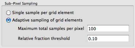
or directly in the ".platform" file within the <capturemethod> section,
<samplestrategy type="adaptive">
  <maxsamples>100</maxsamples>
  <maxfraction>0.10</maxfraction>
</samplestrategy>
In either case, the two defining parameters are:
-
The maximum number of samples that the adaptive sampler is allowed to use. In order for adaptive sampling to have any effect, this number should be somewhat larger than the minimum number of samples allowed — equal to the number of sub-elements defined.
-
The maximum change that is allowed before deciding that the answer has converged sufficiently. This value is described a fractional value that is checked against the relative fractional difference between the new and old radiance values. Since the radiance is a spectral value, the fraction is checked against the extremes in the data array (polarization information is ignored and only the scalar values are used):
\begin{equation*} \mbox{if} |L_o-L_n| / L_o < f, \mbox{converge} \end{equation*}
Background/Approach
The adaptive sample strategy gets its name from the fact that it has to generate samples by adapting to the portion of the scene viewed by a pixel. A scene in DIRSIG exists as an abstract collection of primitive mathematical objects (mostly triangle facets) that are only loosely related to each other as a whole. There is no quick look-up function that might describe the contents of a scene intersected by a detector solid angle (and most practical approaches to that type of problem would involve the same ray tracing techniques that are already being used to sample the scene). Because a sensor can be placed anywhere within a scene and the user has arbitrary control of scene content, this means that the detector model sampling the scene has no useful a priori knowledge of the underlying complexity of what they are looking at. The adaptive sampler must instead use as much knowledge as it has at any given point in time to dictate its next step.
At the start of a pixel problem, the sampler knows two things. First, it knows it needs to find the average radiance corresponding to the sensitive area of the detector projected on the scene. Second, it knows that the user wants that problem to be broken up into a number of sub-problems that are easier to solve (the sub-element grid of the pixel). Since it must use a minimum of one sample per sub-element and it knows the maximum number of samples it is allowed over the entire pixel, the sampler starts by allocating samples to each sub-element based on its relative weight. If the response is uniform, then each sub-element gets roughly the same number of potential samples.
When the pixel has a non-uniform weight function (i.e. when the effective response function of the detector is non-rectangular), samples are "importance" sampled, giving more samples to the more important (highest response) portion of the pixel first. However, each sub-element is guaranteed to get at least one sample even if the response in that region is minimal. This pre-allocation approach was found to outperform allocating samples on the fly since it is easier to balance potential allocations initially than maintain balance as the pixel fills up.
The first sampling step is to "greedily" gather some initial information about the content of each sub-element by generating one sample for each of these regions. Samples are generated "randomly" from a uniform distribution (see Sample Generation), This might look something like:
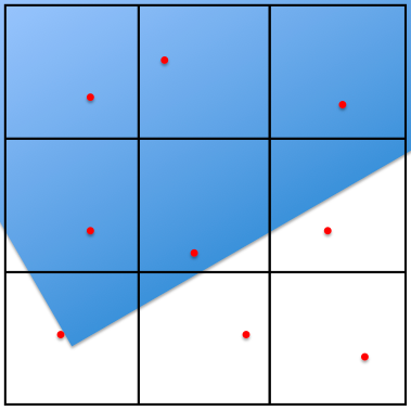
Since we still don’t have any information about variability within each sub-element (just a single radiance value for each), the adapter uses neighborhood information (direct and diagonal sub-elements) to drive a second pass of sampling.
|
|
This document only considers using adaptive sampling for radiance driven simulations. Currently, adaptive sampling only support passive simulations and only the scalar (unpolarized) content of the passive signal. It is intended that the type of approach will be applied to both gated and polarized data at some point in the future. |
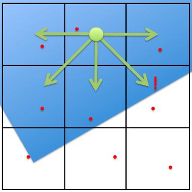
In this second pass, each sub-element with a neighbor that differs from it by the fractional threshold is flagged as needing samples and the sub-element is sampled until the fractional change within it drops below the threshold (or the maximum number of samples is reached).
|
|
When a sub-element has been flagged for getting more than a single sample, it will always get at least 3 samples or one percent of the maximum, whichever is higher. This ensures that we give the sampler a chance to find some variation in the sub-element in cases where we have even the slightest indication that there might be some. |
A third pass occurs (and is repeated) whenever any more than the minimal number of samples were used for a pixel sub-element during the second pass. This pass repeats the whole process, comparing neighbors, looking for differences, and generating more samples for sub-elements that appear to need it. This makes sure that any newly discovered variation in a sub-element gets propagated to its neighbors until the possibilities are exhausted.
Example
This three pass approach has proven to be very robust for passive simulation optimization. The following figure shows the number of samples used for each pixel during a MegaScene1 simulation:
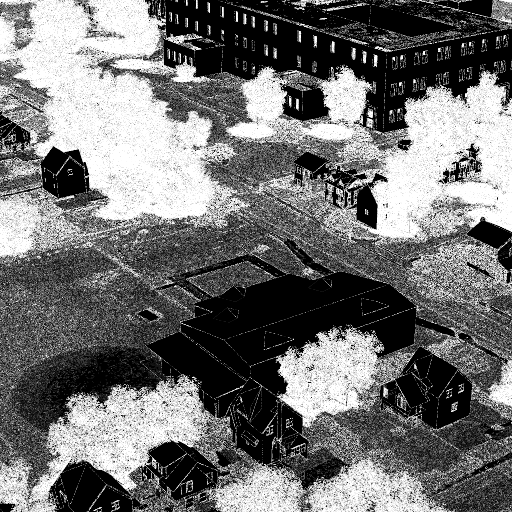
Notice that the trees (the most complex geometric content in the scene) consistently get the maximum number of samples, as do the hard edges of buildings/windows. In contrast, areas with very little variation (such as the house walls and roofs, which have no texture in this simulation) get the minimum number of samples. Moderately varying, textured regions, such as grass and the top of the school building (upper right) are somewhere in between.
Sample Generation
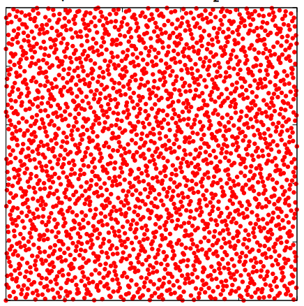
Standard pseudo-random number generators (such as random or drand48) have poor uniformity (and randomness) characteristics under normal operating conditions (see below):
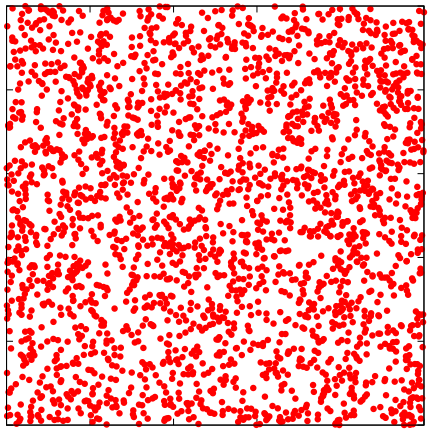
The effectiveness of adaptive sampling is dependent on getting very good coverage of the pixel sub-element. Additionally, since we don’t know ahead of time how many samples we’ll end up using, we need to make sure that we get that uniform coverage no matter how many samples we get. Therefore, instead of using a pseudo-random number generator, adaptive sampling uses a sampler from a class of "quasi-random" number generators with guaranteed uniformity (see Harald Niederreiter. Random Number Generation and Quasi-Monte Carlo Methods. Society for Industrial and Applied Mathematics, 1992). Specifically, we use the Halton sequence, which appears random (though it is actually quite deterministic in generation) and has very good uniformity regardless of when you start/stop pulling samples: