This is the listing of all the demonstrations that are distributed with DIRSIG. A DIRSIG "demo" is simple, stand-alone simulation that is designed to show the user how to use a specific feature in the DIRSIG model. In most cases, the demo scenarios use simple scenes, simple sensors, etc. to convey the point.
How to use a demo
For each demo, there is a link to a local ZIP file (installed with DIRSIG) containing all the files necessary to run the demo. The three easy steps to using demo are:
-
Download the demo,
-
Unpack the demo, and
-
Run the demo
Download the demo
Download the ZIP file containing the demo by clicking the "Download this demo" link at the bottom of the demo summary. Please note that Internet Explorer users might need to select the right-click "Save Target As …" menu item to download the ZIP file into their account.
Unpack the demo
Unzip the demo files into your account (instructions to unzip the archive file are beyond the scope of this document). The demo will be self contained in a folder with the same name as the demo, and the demos are setup to run from where ever the files are placed.
Run the demo
There is a README.txt file in each demo that contains a description
of the demo. To run the demo, simply load the .sim file in the DIRSIG
Simulation Editor and click the Run button.
Static Scene Geometry
Static Instancing Options
This demo is to show different static instancing options available in the ODB and GLIST files. Specifically, this demo was originally created to show how to use the 4x4 "affine matrix" option in the ODB file. It was then expanded to show the same option in a GLIST file. This demo also includes an example of the binary instance file option.
Geolocated Insertion via the GLIST file
Scene geometry and the platform location can be specified using geocoordinates. DIRSIG supports the Geographic (latitude, longitude and altitude), Universal Transverse Mercator (UTM) and Earth-Centered, Earth-Fixed (ECEF) coordinate systems in the GLIST file (to position geometry instances) and the PPD file (to position and orient scene geometry and the platform). This demo includes various examples of geolocated objects and platforms.
Moving Scene Geometry
The following demos describe various ways to include moving geometry in a scene description.
Positioning an object with Delta Motion
This demo shows how to put moving geometry in to a scene using the
Delta motion model.
A car is shown driving across a flat ground plate using a .mov file.
Positioning an object with Generic Motion
This demo shows how to put moving geometry in to a scene using the
Generic motion model.
A car is shown driving in a circle on a flat ground plate using a
.ppd file to describe the position and orientation vs. time.
Positioning an object with Flexible Motion
This demo shows how to put moving geometry in to a scene using the Flexible motion model. A plane is shown flying across the scene with some semi-periodic "roll" (rotation about the along-track or heading axis) that is incorporated using a temporally correlated "jitter" model.
Nested/Hierarchical Motion
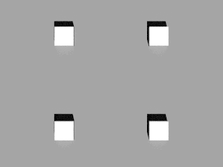
This scene is used to demonstrate nested or hierarchical motion. In the scene, a 2 x 2 grid of balls (spheres) and cube rotate about a central point and that point orbits around a second point.
Sub-object Motion #1
This demo shows how a component of an object can be assigned motion. In this case, the missile on a simple mobile missile launcher is commanded to transition from an erect position to a lowered position. In addition to showing how to associate motion with a part, this demo shows how to change the materials assigned to a part and how a part can be disabled.
Sub-object Motion #2
This demo shows how a component of an object can be assigned motion. In this case, the rotor blades on a helicopter are put into motion using the Flexible motion model. In addition, this demo uses temporal integration on the focal plane (see the TemporalIntegration1 demo for more info) to capture the motion blur on the moving blades.
SUMO-Driven Traffic
This is a baseline simulation that features a traffic pattern produced by the Simulation of Urban MObility (SUMO) model. All the input files for both the SUMO simulation and the DIRSIG simulation that ingests the output of the SUMO simulation are included. This is not intended to be a detailed tutorial on using SUMO itself, as there is a wealth of existing documentation, tutorials and examples available on the SUMO website.
Built-in Scene Geometry
Built-in Pile Objects via the ODB file
This scene shows some of the built-in geometry objects that can be used to form various types of "piles".
Built-in Geometry Objects via the ODB file
This scene demonstrates a set of the built-in geometry objects available in DIRSIG. The scene is constructed using an ODB file.
Built-in Geometry Objects via the GLIST file
This scene demonstrates a set of the built-in geometry objects available in DIRSIG. The scene is constructed using a GLIST file, which has an expanded set of built-in objects (compared to the ODB file) and allows the built-in objects to be instanced.
Reference/Calibration Geometry
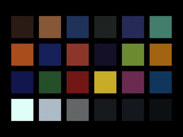
Macbeth Color Checker
This demo contains a bundled object version of a Macbeth Color Checker. This object can be easily inserted into other scenes and used to create color calibrated images from DIRSIG’s native radiance images.
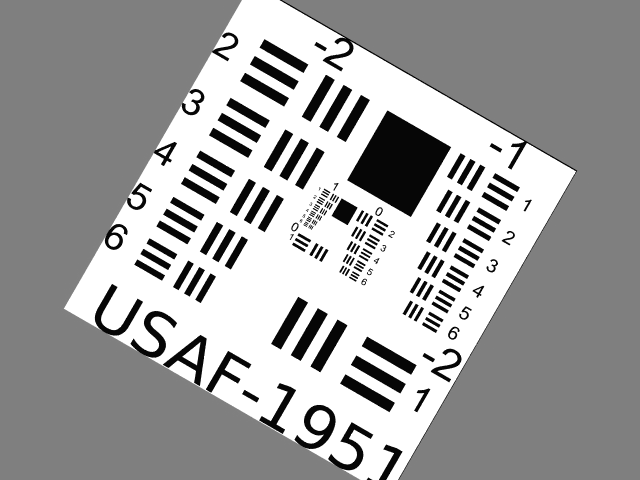
USAF Resolution Target
This demo contains a bundled object version of a USAF Resolution Target. This object can be easily inserted into other scenes and used to to characterize the resolution of the sensor imaging the scene.
Advanced Scene Geometry
Object and Instance Material Overrides
This demo shows how to utilize material overrides at the object and instance level. The scene features multiple static and dynamic instances of the same car with each instance overriding the body paint color assigned in the base geometry. This introduces more options for efficiently sharing base geometry across instance with unique material attributions.
Basic Vertex Normals
DIRSIG supports vertex normals in OBJ geometry files. In these files, a normal vector is associated with each vertex. DIRSIG spatially interpolates this vertex normal information across a polygon surface at run time.
Vertex Normals and Sun Glints
This demo provides examples for modeling sun glints off vehicles when the geometry and radiometry models are properly configured. For the geometry, two versions of the same vehicle are used. One has a single normal vector for each facet, while the other has a normal vector associated with each vertex. In the second case, vertex normal interpolation is employed, which continuously varies the normal across the facet. This minimizes the artifacts of using quantized geometry for a continuous surface and produces more realistic solar glints.
Using Decal Maps to Drape Geometry
This demo shows how to use a special kind of map to drape one set of geometry onto another. This is very useful for geometry that needs to follow the surface of another. In this demo, some road geometry is mapped onto an undulating surface.
Using a Polygon to Auto-Populate Objects
The motivation for the polygon based random fill is to allow constrained areas of a scene (such as backyards or rooftops) to be randomly filled with similar items. In contrast to some of the other methods of doing this (such as basing it on a material map or density map), the polygon fill ensures that the same random placement is done individually for each polygonal area, which guarantees more uniform global statistics and speeds up sparsely filled areas.
Using Density Maps to Auto-Populate Objects
The density map based random fill lets you take advantage of the mapping mechanisms to define populated areas that vary in density of the surface of an object. This can be useful in cases where you know roughly where objects should be, but don’t want to define specific locations nor want them to be uniformly placed either.
Using Base Geometry and Material Populations #1
This demonstration focuses on mechanisms added to the GLIST file to facilitate rapid scene development based on (1) randomly created populations of base objects and (2) variations in material attribution for those base objects.
Using Base Geometry and Material Populations #2
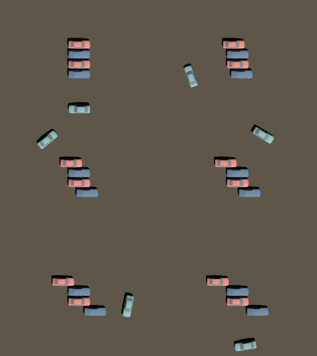
This example shows how a parking lot can be filled with cars using a small set of base geometries (different car models) and materials (different paints) to automatically generate a population of car variants. In addition, this demo also leverages some of the tools to the position cars generation from that population within the lot and place shopping carts between them.
Pre-Packaged Materials
This example shows a prototype capability for packaging (bundling) materials. This technique should pave the way for creating databases of materials, with each represented by a single file that contains all the optical and thermodynamic data for the material. These files can then be mapped into a scene or bundled object from a central repository with minimal effort.
Bundling Materials and Maps with Geometry
This example shows how to create "bundled objects", which are folders that contain geometry and all the material and maps (material, texture, etc.). This approach allows collections of fully attributed objects to be created that can be injected into scenes without any need to manually merge material properties.
Bundling Sources and Motion with Geometry
In this night scenario, a "suspect" car is stationary in a parking lot and a police car approaches (with headlights and spinning lights) and stops. This demo utilizes the "bundled object" approach that allows objects to be encapsulated into folders that contain all geometry, material properties and maps (material, texture, etc.).
Multiple Scenes
This demo shows how multiple scene databases can be combined at run-time. This feature allows multiple scenes to be tiled together or overlaid in an effort to simplify and streamline scene construction and management. In this case, a modular city is assembled from 30 "block-sized" elements.
Total Solar Eclipse
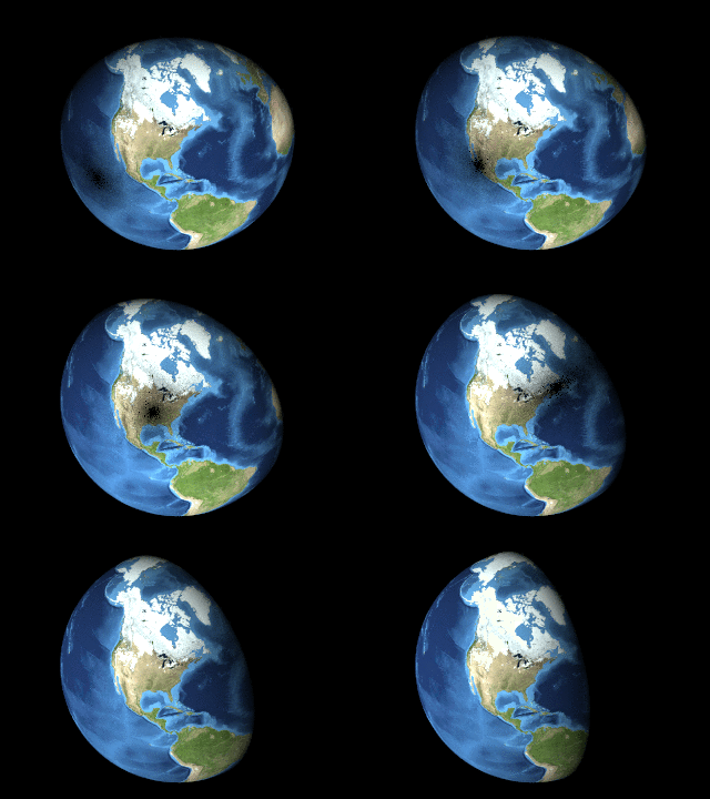
This demo simulates the North American total solar eclipse that occurs on April 8th, 2024. A solar eclipse occurs when the moon transects the sun and casts its shadow on the earth. This DIRSIG simulation models the earth via the EarthGrid plugin and models the moon as an appropriately sized sphere that orbits the earth using the FlexMotion model driven by ECEF coordinates extracted from an external simulation using NASA’s SPICE Toolkit. The point of the simulation is to highlight the global positioning of the sun (via the SpiceEphemeris plugin), the global positioning of the moon and the appropriate interaction of the sun and moon.
Optical Properties
The following demos describe methods to configure various optical properties for materials in scenes.
Advanced BRDF Examples
This demo contains examples for how to configure BRDFs for different types of man-made materials with strong directional reflectance properties.
Data-Driven BRDF Example
This demo contains an example of the data-driven BRDF model at the core of DIRSIG5, but which was back-ported to DIRSIG4 for comparisons and DIRSIG4 utility. It stores the BRDF using a spherical quad tree (SQT) data structure, which has some unique and powerful features including adaptive resolution (level of detail), efficient storage, efficient hemispherical integration and efficient sampling mechanisms.
Surface Roughness Example
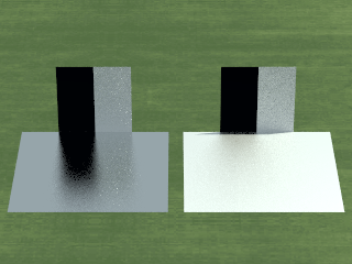
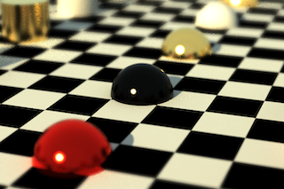
This demo shows how the surface roughness parameter in the parametric Priest-Germer BRDF model impacts the reflections of nearby background objects.
Extinction Examples
This demo shows how to model a variety of volumes (using the built-in primitive geometry) with unique spectral extinction properties and temperature. Primitive volumes are handled a bit differently than RegularGrid objects in that overlapping primitives do not "sum" in term of the concentration of medium materials. Instead, primitive define distinct regions in which the volume itself matches that primitive’s definition exclusively.
Property Maps
UV Mapping with Built-in Geometry
This demonstration shows the UV mapping functionality. Instead of tiling property maps along the horizontal (X-Y) plane, they can be "wrapped" around geometry. The built-in sphere object has a default UV mapping associated with it. The facetized box geometry has a UV coordinate associated with each vertex.
UV Mapping with OBJ Geometry
This demonstration shows a more advanced UV mapping example using an OBJ geometry model and a material map.
Bump Map on a Sphere
This demo shows how to use a bump map to introduce normal fluctuations within a surface.
Bump Map on a Plane
Another demo showing how to use a bump map to introduce normal fluctuations within a surface.
Simple Normal Map
This demo focuses on the use of normal maps to emulate high resolution surface topology on low resolution geometry models. Similar to bump maps, a normal map can be used to spatially modulate the surface normal vector across an otherwise flat surface. This is accomplished by encoding the XYZ normal vector into an RGB image. In this example, a pair of real 3D objects (a hemisphere and a truncated pyramid) are featured and a second pair of the same objects are emulated using a normal map.
Tangent Normal Map
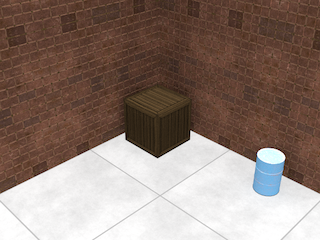
This demo includes several objects that utilize tangent space normal maps that are defined relative to the surface rather than the object’s local coordinate system. In this example, the same normal map is applied to the sides of a wooden crate, which requires the map to be rotated into the coordinate system relative to each side rather than be interpreted in the coordinate system of the entire object.
Material Map
This demo provides a basic example of a material map, which is a tool that employs a raster image to map different materials to different locations on an object. This demo specifically highlights the setup of a material map and the impact of the "pure" vs. "mixed" material option.
Material Map with Holes
This demo provides an example of a material map configuration that includes a "null" material, which creates a "hole" in the surface. The demo includes a camouflage net supported by spreader poles over an HMMWV vehicle, which uses a material map to distribute different color fabrics and empty space across the surface of the continuous net mesh.
Reflectance Map
This demo provides a basic example of a reflectance map, which is a tool that allows the user to use a spectral reflectance cube (perhaps derived from a calibrated sensor) to define the hemispherical reflectance of a material. This is a useful mechanism to incorporate a measured background into a scene.
RGB Reflectance Map
This shows how to use RGB image maps to drive the reflectance on a surface. In this case a sphere object is mapped with an RGB image of the Earth. Note that this technique results in materials that are limited to the visible region since information about the reflectance outside of this region are unknown.
Direct Curve Map
This demo includes examples of using the CurveMap and ENVI Spectral Library (SLI) files to define scene objects with spectral variability. The scene contains a Macbeth Color Checker type panel that is flanked by a pair of grass patches. The left patch is modeled with the classic DIRSIG texture method and the right patch emulates it with a CurveMap.
Mixture Map
This demo utilizes a mixture (or fraction) map to describe the materials on a terrain. The original map was created in Maya and stored as an RGB image, where the three 8-bit channels encoded the relative contribution of three materials at each location. This 24-bit mixture image was converted to a 3 band, floating-point image that DIRSIG expects as input.
Temperature Map
This demo shows how to use a raster image to define the temperature of an object. In addition to including a static scenario (temperatures that do not vary with time) this demo includes a dynamic scenario where the temperatures vary with time using a series of raster images.
Water
Water plugins for a static surface and IOP_MODEL poperties
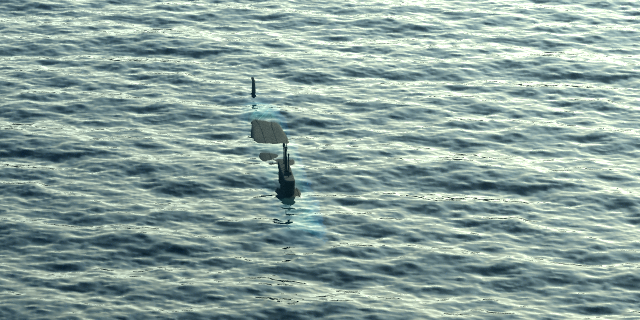
This scene starts to introduce the water plugins for DIRSIG5 and demonstrates the new radiative transfer engine in the context of caustics formed at the bottom of a stepped pool (for the clear water scenario). Two scenarios are provided, a turbid water case and a clear water case.
Water plugins for a external dynamic surface models
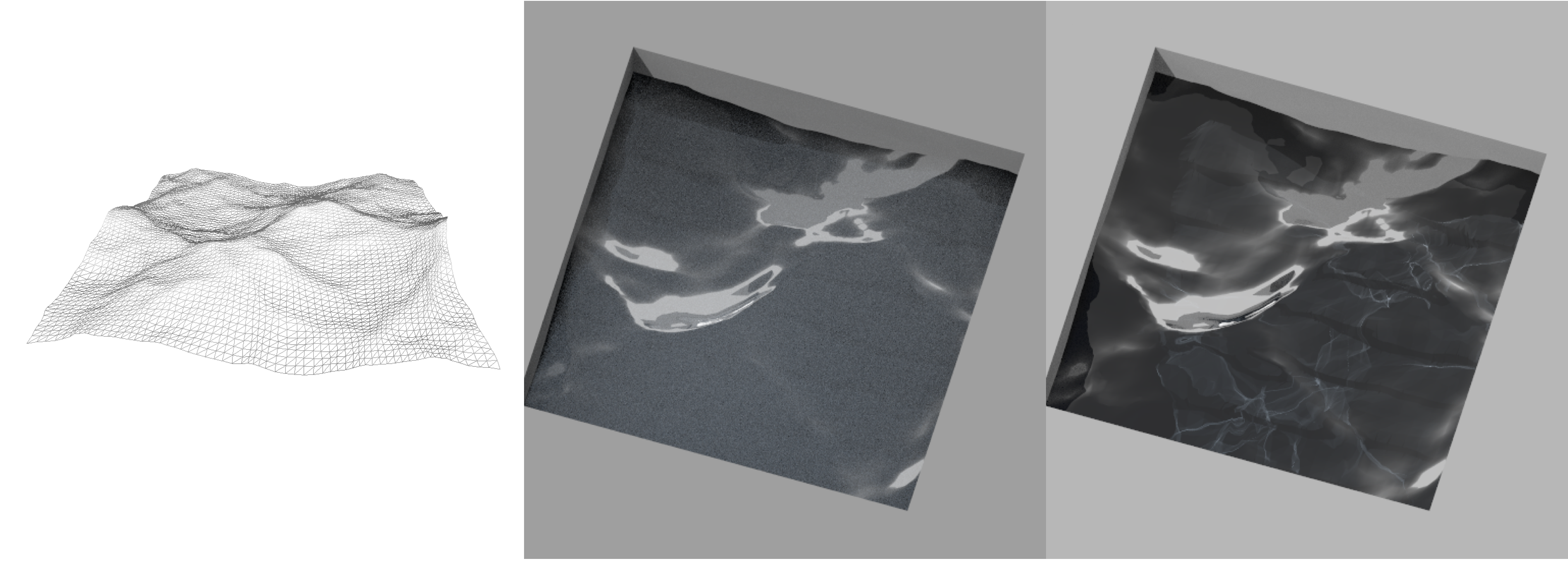
This example shows how to use the HDF medium interface plugin to describe a water medium in DIRSIG. In contrast to an OBJ based interface (see the Caustics1 demo), the HDF interface is intended to bring in external data from arbitrary wave models and to extend that data in both time and space.
Atmosphere
Refraction
This demo shows how both atmospheric refraction and dispersion can be enabled for any classic atmosphere in DIRSIG5 using one of six built-in models. When using the NewAtmosphere toolchain, the refraction can driven by the atmospheric model (e.g. MODTRAN).
Mid-fidelity Four Curve Atmosphere
This demo shows how to both use and construct the database for the
FourCurveAtmosphere
plugin. This plugin provides a higher fidelity atmospheric representation
than the DIRSIG4-era (DIRSIG5
BasicAtmosphere
plugin) SimpleAtm and
UniformAtm models, but lower fidelity than ClassicAtm or
NewAtmosphere.
The original goal of this model is to provide physics-driven atmospherics for
the ChipMaker plugin,
without spending 10x the image generation time computing a traditional
atmospheric database.
Background Sky Contributions
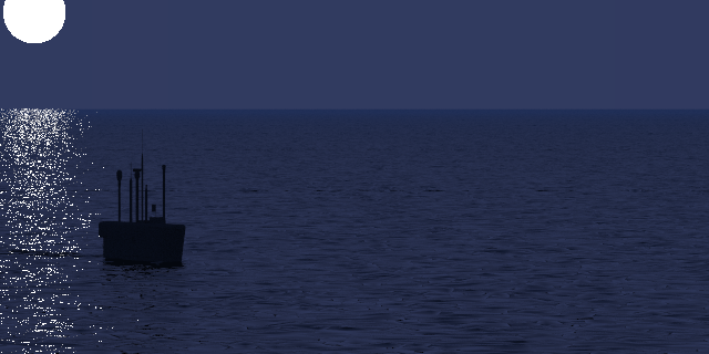
This demo shows how to configure the BackgroundSky plugin to include a hemispherically integrated spectral sky irradiance in a simulation in addition to the sky contributions provided by the atmosphere model. The goal of this tool is to provide a means to introduce additional sky radiance contributions that are not accounted for by the primary atmosphere model. Examples include starlight, airglow, scattered light from a nearby city/town, etc.
Weather Plugins
This demo shows how to configure the various weather plugins in DIRSIG5.
Compatibility 

Clouds and Plumes
OpenVDB Plumes
OpenVDB Clouds
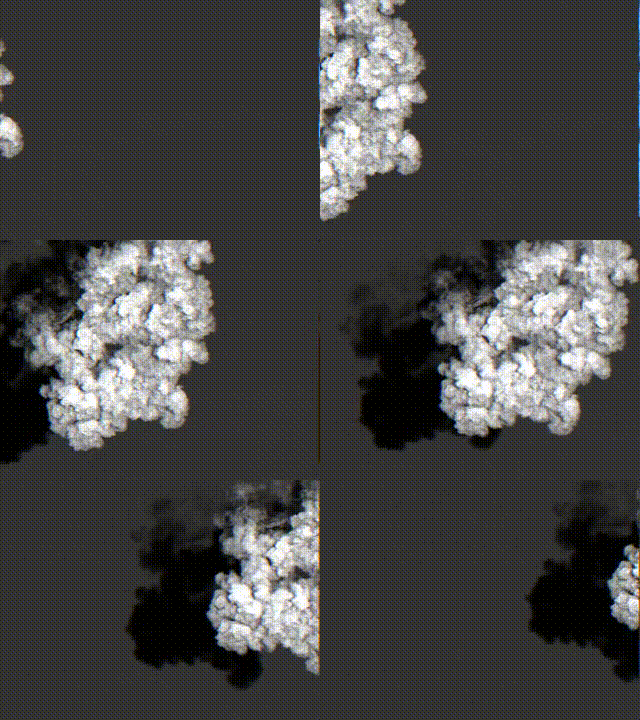
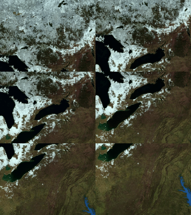
This demo provides a working example of the CloudVDB plugin in DIRSIG, which allows the user to import a cloud using the using the OpenVDB voxel description. Cloud modeling is usually concerned with absorption and scattering at visible wavelengths and absorption and emission at thermal wavelengths (due to water vapor and ice crystals).
Wide-Area 2D Clouds
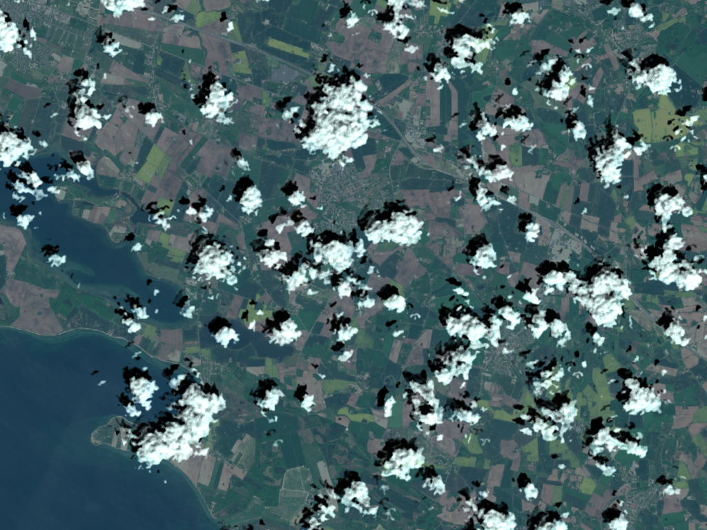
The FastClouds plugin is meant to address the problem of effectively defining very large, high altitude objects that might represent clouds over many kilometers. Over a significant distance, we expect a flat plate to deviate from a constant altitude due to the underlying curvature of the Earth. Instead, the plugin adapts to the WGS84 ellipsoids to maintain a constant altitude and generates a 2D representation of clouds based on an input cloud fraction map. The clouds being modeled by this plugin are intended to be generally opaque (with some transmission at the edges) and as such are modeled as varying between a nominal opaque cloud spectral reflectance and a free path to the Earth. Given their two dimensional nature, these clouds are intended to be viewed from a distance and well above the clouds themselves.
3D Fast Clouds
This demo provides a working example of the fast clouds which allows the user to import a cloud field using the regular grid mechanism, assign volumetric materials to it and use the "fast" cloud radiometry solver. This feature to model clouds is explicitly called the "fast" cloud model because the radiative transfer within the cloud uses a direct solution for first order scattered solar radiance and approximates multiple scattering contributions. It is intended primarily for producing the effects of large-scale clouds on a scene (particularly shadowing), but not for accurate, detailed radiometry of the clouds themselves.
2D Fast Clouds
This demo shows how to utilize 2D cloud maps to emulate thin (e.g. cirrus) clouds. This can be accomplished with either a material map with mixing or a full mixture map.
Reflected Sky with a cloud "mask"
This demonstration is a modification of Skyview1 demo that demonstrates the use of cloud "masks" to approximate the angular distribution of cloud irradiance across the sky dome (the "clouds" are not physical objects and use a simple spectral model for approximate behavior in the visible/NIR only). It is useful for studies looking at the impact of non-uniform cloud fields on reflected signal (e.g. from the ocean surface), but is not intended for absolute radiometry work.
Voxelized Geometry
This demo provides the user with an example of how to import a volumetric object (for example, a 3D plume, cloud, etc.) into DIRSIG. In this example, a 3D model of a flame is imported from an external model that provides gas density and temperature information.
Radiometry
Leaf Stacking Effect
The scene is composed of a background over which a stack of successively smaller "leaf planes" is placed. These "leaf planes" have a material optical properties that approximate those of real leaves. The impacts of the spectrally varying transmission at different wavelengths is then observed.
Reflected Sky
This demonstration contains a mirrored hemisphere that reflects what a MODTRAN-driven sky irradiance field looks like at 8:10 AM local time. The mirrored hemisphere employs a unique material description to make a surface that is a perfect mirror and can be efficiently modeled by DIRSIG.
Reflectance Inversion
This scenario is supposed to demonstrate how the reflectance of a surface can be inverted from a spectral radiance image and an Atmospheric Database (ADB) file.
Secondary Sources
Please consult the User-Defined Sources Manual for more information.
A Point Source
This demo shows users the basic configuration of secondary sources. The supplied files place an array of different point sources over a simple background.
An Indoor Source
This demo models an indoor scene that contains a point source near the ceiling of a room featuring simple cut-out window and door (with no glass). Interior illumination is provided by both the source and the window.
Instancing Sources
This demo shows how to instance sources with other geometry in a scene. In this case, we have a vehicle with headlights. A single point source is instanced to make the two headlights and bundled with the vehicle geometry. Then the vehicle geometry is instanced in the scene, pointed in two directions and given some dynamic motion.
Blinking/Modulating Sources
This demo shows how to setup temporally varying sources. In the scene, a combination of blinking and modulating sources are setup. One is always on, two use the "blinking" parameters (frequency and time offset) and three are assigned power spectral density (PSD) descriptions to define modulation. To represent what might be observed in a large area with a 3-phase power grid, the three modulating sources are out of phase with each other by 120 degrees. The scene is then observed with a 2D array camera employing a 2400 Hz read-out rate so that the modulation of the AC sources can be observed.
Advanced Source Shaping
This demo focuses on how to setup point sources with multiple shaping coefficients, which allows the user to create more complex angular intensity patterns verus a single shaping coefficient. The scene consists of an array of point sources illuminating a flat surface. The scene has two rows containing 3 types of sources: (1) a wide beam source, (2) a narrow beam source and (3) a combination wide and narrow beam source. One row has each source illuminating the underlying flat surface horizontally. The other row has the same sources illuminating the surface from a vertical direction.
IES Source Shaping
This demo describes an alternate source shape format based on the IES (Illuminating Engineering Society) standard. It is not meant as a full lighting description (IES only has human eye relative, photometric data). Instead, only the shape of the source is read and combined with the usual source definition (see Sources1).
Commanded Sources
This demo shows how GLIST tags and a control file can be used to dynamically enable/disable sources in a scene. In this example, a system of lights (headlights, taillights, brake lights, turn signals) have been added to a car and they are turned on and off as function of time.
Platform Mounts
Please consult the Instrument Mounts guide for more information.
Commanded Mount (Rotation)
This shows how to setup the directly-commanded mount, which allows the user to specify non-periodic, platform-relative pointing angles as a function of time.
Commanded Mount (Translation)
This shows how to setup the directly-commanded mount, which allows the user to specify non-periodic, platform-relative translation as a function of time.
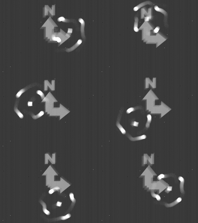
Lemniscate Scan Mount
This setup demonstrates how to use the "Lemniscate" mount to drive figure-8 style, platform-relative scanning.
Line Scan Mount
This setup demonstrates how to use the "line" mount to drive unidirectional, linear velocity, platform-relative scanning in the nominal across-track direction.
Tabulated Mount (Rotation)
This setup demonstrates how to use the "tabulated" mount object to drive platform-relative scanning using measured or externally generated rotation data.
Tabulated Mount (Translation)
This setup demonstrates how to use the "tabulated" mount object to drive platform-relative scanning using measured or externally generated translation data.
Tracking Mount
This demo shows how to use the "tracking" mount to always point at a specific target geometry instance. This mount dynamically accounts for both platform and target motion. It is useful for setting up scenarios such as a UAV with a camera ball that follows a vehicle.
Scripted Mount
This demo shows users how to use the "scripted" mount object to drive platform-relative scanning that is driven from a user-supplied script.
Whisk Scan Mount
This setup demonstrates how to use the "whisk" mount to drive bidirectional, sinusoidal, platform-relative scanning in the nominal across-track direction.
Platform Motion
Temporally Uncorrelated Jitter
We take what would otherwise be a non-moving, down-looking platform and jitter its position as a function of time using a normal distribution.
Temporally Correlated Jitter
We take what would otherwise be a non-moving, down-looking platform and jitter its position as a function of time using a temporally-correlated function.
STK Import
This demo shows how to ingest mission planning reports produced by
Systems Toolkit (STK).
Specifically, how the DIRSIG
FlexMotion model can
directly read STK ephemeris (.e) and attitude (.a) reports. This
demo is also "scene-less", in that it doesn’t use a conventional DIRSIG
scene and utilizes the
EarthGrid plugin
exclusively for the scene.
Advanced Platform Concepts
Multiple Camera Payload
This demo which features four cameras on a single platform. Each cameras has a different attachment affine transform so they point in different directions with some overlap between all the cameras. DIRSIG automatically includes basic image geolocation information in the output ENVI header file, so the separate images can easily be mosaiced via standard software packages.
Data-Driven Color Filter Array (CFA)
This demo shows how to use the data-driven focal plane feature to model a Bayer pattern focal plane. The output is a single-channel image containing the mosaic’ed red, green and blue pixel values.
Built-in Color Filter Array (CFA)
This demo shows how to generate raw, mosaiced output of a color filter array (CFA) that can be demosaiced by the user. This demo includes example setups for both Bayer and Truesense CFA configurations.
Data-driven array with non-linear gain
This demo shows how to use the linear and non-linear gain models available with the data-driven focal plane array feature. The 2D array sensor looks at a scene containing 5 panels spanning a range of reflectances. The upper half of the array is assigned a linear gain model. The lower half of the array is assigned a non-linear gain model that maps the brightness of the two darkest and two brightest panels to the same value. Beyond the basic linear and non-linear effects shown here these gain models can be used to create transfer functions that convert the radiometric units normally output by the model into integer digital counts. Such transfer functions can account for the optical throughput of the optical system, the quantum efficency of the detectors, on-chip amplification, off-chip amplification, etc.
Data-Driven Clocking
This demo shows how to drive a "clock" object with external (and potentially irregular) trigger times. In this case, the camera is imaging a "clock-like" scene with hands moving at a constant angular rate. One scenario images the clock with a constant readout rate, which results in images of the hand making regular process. The second scenario images the clock with an irregular readout rate, which results in a series of images where the hand makes abrupt jumps between frames.
Temporal Integration (Scene Motion)
This demo describes how to enable temporal integration of pixels. This allows motion blur from scene object and/or platform motion to be included in the output data product. Although this demo focuses on motion blur of a fast moving object being captured by a 2D framing array camera, this feature can also be used to model many aspects of a time-delayed integration (TDI) focal plane, including the pushbroom architectures used in many remote sensing imaging platforms.
Temporal Integration (Platform Motion)
This demo describes how to enable temporal integration of pixels. This allows motion blur from scene object and/or platform motion to be included in the output data product. This demo complements the TemporalIntegration1 demo. In that demo, the platform is fixed and the car in the scene is moving. In this demo, the platform is moving and the car in the scene is fixed. In both cases, the car looks blurred due to the relative motion between the car and platform.
Rolling Shutter with Integration
This demo shows how a focal plane can be configured with a rolling shutter, where each line (row) of a 2D array is integrated and read out sequentially. In contrast to a global shutter (where all rows are read out at once), the rolling readout produces artifacts in the image when motion is present in the scene at frequencies proportional to the rolling shutter line rate. In this case, we are looking at a spinning rotor on a helicopter.
Sub-Pixel Object Hyper-sampling
This demo shows how to improve the modeling of sub-pixel objects by enabling hypersampling when a pixel’s IFOV contains specific objects. The scene constains a pair of very small box targets that represent a fraction of a percent of the pixel by area. However, even with modest sampling across the array the correct fractional contribution of these small targets can be determined when hypersampling is enabled.
Sub-Pixel Feature Hyper-sampling
This simulation demonstrates the use of hypersampling to improve sampling in a large (many pixels) object that has a small (sub-pixel) component that is important. In this case, we have a moving vehicle that has a hot spot on the hood that is important to sample well. Failure to sample it could result in a flickering effect from frame to frame as some frames have sampled this high-magnitude component well and others have not.
MicroBolometer Camera
This demo focuses on a sensor configuration to approximate the response and commonly observed artifacts of a microbolometer camera system. This demo leverages the built-in detector model in the BasicPlatform sensor plugin to model a camera with a broad LWIR spectral response, a long decay (response) time, dead and hot pixels and fixed pattern noise.
Lens Distortion
This demo shows how to use the lens distortion model in the DIRSIG5 BasicPlatform sensor plugin. This feature allows you enhance the pinhole camera approximation employed by this sensor plugin with a common parametric lens distortion model that allows the user to introduce common distortions including barrel, pin cushion, etc.
Time-Delayed Integration
This demo shows how to configure a 2D array as a 1D pushbroom array with multiple stages of time-delayed integration (TDI) in the DIRSIG5 BasicPlatform sensor plugin. Time-delayed integration (TDI) is a strategy to increase signal-to-noise ratio (SNR) by effectively increasing the integration time for each pixel. Rather than using a single pixel with a long integration time, TDI uses a set of pixels that will image the same location over a period of time.
Finite Focus Distance
The BasicPlatform plugin is typically used to simulate cameras that can be modeled using a pinhole camera approximation that are focused at inifinity. This demo shows how to specify a finite focus distance in a camera modeled by the plugin, which triggers an advanced sampling of the user-defined aperture. The camera is placed at a slant angle and the focus distance is set to focus on objects in the center of the image frame. Due to the low F-number of the camera (f/1.1), the depth of focus is very small, resulting in objects in the foreground and background being out of focus.
Telecentric Lens Scenario
This demo includes a basic example of setting up a telecentric lens using the basic platform plugin. The paths cast from each pixel enter the scene bound by a maximum telecentricity angle (0 deg being straight out). In this demo two spheres are place at varying distances from the camera. With pinhole projection, the sphere further away would appear smaller. With telecentric projection, they appear the same size.
Alternative Sensor Plugins
Single Scene Image Chip Sets for Machine Learning
In order to facilitate robust training of machine learning algorithms, we want a large number of images featuring the content of interest. These image "chips" should span a wide range of acquisition parameters. This plugin was created to streamline the generation of image chips with "labels" by automating the sampling of a user-defined parameter space in a single simulation rather than relying on an infrastructure of external scripts to iterate through the parameter space.
Multi Scene Image Chip Sets for Machine Learning
This is demonstration of the ChipMaker comboi plugin with an alternative scene model approach that leverages a collection of smaller area background scenes (referred to as scene-lets) and a collection of target scenes that are combined on-the-fly to facilitate greater variation of targets and backgrounds.
Point Collectors
This demo provides a working example of the PointCollectors sensor plugin. This plugin allows the user to arbitrarily place a number of point radiometers in the scene and they can be configured to collect in a variety of modes. This type of sensor can be useful for measuring the illumination within a scene as either a function of location, time or both.
Spherical Collector
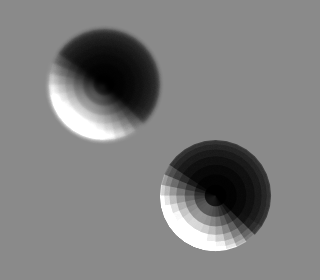
This demo shows how to use the SphericalCollector sensor plugin, which allows the user to easily collect data from a sphere or hemisphere around a point in space. The plugin supports both ortho and polar projections as well as "inbound" (looking outward at the radiance arriving at the specified point) and "outbound" (looking inward at the radiance leaving the specified point).
Virtual Goniometer
This demo shows how to use the SphericalCollector sensor plugin to emulate a goniometer used to measure bi-directional reflectance distribution (BRDF) functions of surfaces. In this scenario, a surface is populated with a distribution of spheres that are illuminated from a single direction and the sensor plugin captures the light scattering into the hemisphere above the complex surface.
Thermal
The following demos pertain to modeling the thermal regions of the EO/IR spectrum.
THERM Temp Solver
This scene demonstrates various ways to assign temperature to objects in a DIRSIG scene, and the units required on the input side.
Dynamic Shadows with THERM
This demo shows how the built-in THERM thermal model can model temporal shadow signatures. In this scenario, we have a simple scene with two boxes that we observe over a period of an hour. During that hour, the high thermal inertia background responds to the solar shadowing created by a stationary box (left) and a box that moves to a new location (center → right).
Dynamic Heating and Cooling with THERM
This demo shows how the built-in THERM thermal model can model dynamic heating and cooling conditions. In this scenario, a pair of aircraft are repositioned. The first plane has been parked all day and then pulls forward to reveal thermal shadow "scar" on the concrete. A second, identical plane has been inside the hangar all day and then pulls forward into the sunlight to reveal its cooler surface temperatures. After the two planes quickly reposition, the simulation captures a series of frames over the next hour. During that hour the shadow left by the first plane slowly fades, the second plane heats up and new shadows develop beneath both planes.
Data-Driven Temp Solver
This demo shows how the data-driven temperature solver and an external temperature vs. time file can be used to drive the temperature of an object in a DIRSIG simulation. In this demo, a simple utility pole with three transformer "cans" is constructed. One of the transformer "cans" is passively heated by the Sun (using the built-in THERM temperature solver) and the remaining two are driven by unique temperature vs. time data files. The simulation generates an LWIR image every hour over the course of a 24 hour period so that the variation in the various objects can be observed.
Balfour Temp Solver
Mapped Balfour Coefficients
This demo shows how to spatially map Balfour coefficients to produce
background temperature variation. It also shows how shadows affect
Balfour temperature model predictions. Since this capability is
unique to DIRSIG5, it also shows how to use python and h5py to
modify the scene HDF output by scene2hdf to introduce Balfour
maps to scenes.
Expanding Fireball
This demo shows how to model a expanding fireball with dynamic temperatures. The fireball is modeled as an analytical (primitive) sphere and a DeltaMotion description to change the size (via scales) as a function of time. The dynamic temperature uses the DataDrivenTempSolver to vary the temperature vs. time.
Mapped THERM Properties
For a given material, the parameters fed in to the THERM temperature solver can be spatially varied using a property map image. This demonstration drapes such a property map over a terrain geometry.
Import MuSES Results
This demo shows how the import results from the MuSES temperature prediction and infrared signature model developed by ThermoAnalytics, Inc. DIRSIG can import both the geometry and the temperature results stored in a MuSES TDF file.
Compatibility 

|
Important
|
MuSES support is only available on Windows and Linux. |


MuSES Integration
This demo shows how setup DIRSIG to run the MuSES temperature prediction and infrared signature model developed by ThermoAnalytics, Inc. on-the-fly. The MuSES plugin for DIRSIG will make sure to sync the conditions between DIRSIG and MuSES (e.g., geographic location, date, time, weather, orientation), run MuSES and then read the temperature results and MuSES material properties in. The plugin supports having multiple MuSES targets and/or multiple instances of the same target(s) in a single DIRSIG simulation.
Compatibility 

|
Important
|
MuSES support is only available on Windows and Linux. |

Temperature Map
See the demo in the Property Maps section.
LIDAR
Please consult the Lidar Modality Handbook for more information.
Nadir Looking, Single Pulse Example
This demonstrates a nadir viewing (down-looking) LIDAR system. In this case, we only shoot a single pulse at a tree object.
Whisk Scanning, Multiple Pulse Example
This demonstrates an airborne, whisk scan LIDAR system. The platform remains still while 5 pulses are sent and received in a simple scan pattern.
Side Looking, Single Pulse Example
This demonstrates a side-looking LIDAR system, like one that might be mounted on a vehicle driving down the street and mapping the side of buildings. In this case, we only shoot a single pulse.
Nadir Looking, Advanced GmAPD Example
This demonstrates a nadir viewing (down-looking) LIDAR system using the Advanced GmAPD detector model. In this case, we only shoot a single pulse at a tree object.
Side Looking, Advanced GmAPD Example
This demonstrates a side-looking LIDAR system looking at a far off object. It also outlines the use of the Advanced GmAPD model to produce ASCII/Text Level-0 (time-of-flight) style data.
Whisk Scanning, Advanced GmAPD Example
This demonstrates a nadir viewing Geiger-mode Avalanche Photo-diode (GmAPD) laser radar system that whisk scans across the scene. The collection shoots 40 overlaping pulses over a scene composed of a tree on a background.
Bi-Static Collection
This demonstrates an exaggerated LASER offset in a LIDAR system. In this case, we shoot a single pulse from a greatly offset laser (one that 2km behind the focal plane) and angled such that is is illuminating the space vertically underneath the sensor. The primary reason for this demo is to show a laser instrument that is completely independent from the gated focal plane instrument (they are on different mounts in the platform).
Multi-Static Collection
This demonstrates a multi-static (multi-vehicle) collection scenario. It features a single transmitter and two receivers distributed on three separate vehicles.
Compatibility 

Retroreflection Return
This demonstrates the strong retro-reflection of the lidar pulse by a corner retroreflector object in the scene. This demo highlights the efficient multi-bounce calculations used in DIRSIG5. This scenario is difficult to correctly configure in DIRSIG4.
Sloped Surface Return
This demonstrates the broadening of a return from a sloped surface. The demonstration includes simulations of returns from both a flat (perpendicular to the beam) and sloped (not perpendicular to the beam).
Multi-Return Waveform Example
This demonstrates multiple returns from multiple objects (at multiple ranges) within a pixel. Specifically, this demo focuses on correctly configuring the pixel sub-sampling to achieve a realistic waveform.
Link Budget Verification
This is a LIDAR verification/validation demonstration. An Excel spreadsheet is included which shows a hand-computed, "expected" result which can be compared against the DIRSIG output.
Dynamic Range Gate
This demo shows how the user can drive a LIDAR simulation with external range gate data.
Compatibility 

Incorporating Command and Knowledge Errors
This demo shows how the user can incorporate command errors (for example, jitter) and knowledge errors (for example, GPS or INS noise) into a LIDAR simulation. This demonstration includes 4 scenarios to explore the various combinations (with and without) of both command and knowledge errors.
User-Defined Spatial Beam Profile
This demo shows how the user can drive a LIDAR simulation with a user-defined spatial beam profile. In this case, the beam is an approximation of a TEM22 beam, created from a 3x3 grid of Gaussian beams.
User-Defined Temporal Pulse Profile
This demo shows how the user can drive a LIDAR simulation with a user-defined temporal pulse profile. This demonstration includes two simulations: (a) a "clean pulse" scenario with an ideal Gaussian pulse profile and (b) an "after pulse" scenario that features the same primary pulse but also includes a lower magnitude after pulse that is 10% of the magnitude of the primary pulse and time shifted by 5 ns.
Polarization
The DIRSIG5 roadmap does not include supporting polarization. DIRSIG4 will continue to be available with polarization support.
Basic Reflective Polarization
This scene demonstrates two of the BRDF models available in DIRSIG. The "chunky bar" (four flat-topped pyramids on a plate) has different roughness aluminum materials applied to each pyramid. The metal uses the Priest-Germer pBRDF model. The plate has a grass material applied, and uses the Shell Background model.
Thermal Polarization
This demonstration is for simulating a thermal infrared, polarized system. The scene is similar to the "Beach Ball" scene described in Mike Gartley’s dissertation.
Division of Aperture Polarization
This is a 4-camera "division of aperture" setup using the Modified-Pickering 0, 45, 90 and 135 filter set.
Compatibility 

Division of Focal Plane Polarization
This is a single focal plane using a 2x2 micro-grid "division of focal plane" setup using the Modified-Pickering 0, 45, 90 and 135 filter set.
Compatibility 

Space Domain Awareness (SDA)
Please note that using DIRSIG for SSA applications is still experimental. Please consult the SSA Modality Handbook for more information about current features and limitations.
Ground to Space ("Moon Sat") Scenario
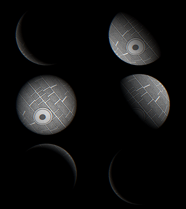
This is a DIRSIG4 demonstration of looking at an exo-atmospheric object from a ground based sensor. In this case the object is an object that looks like the Moon (but is much smaller at only 16.8 km meters across) in a geo-synchronous orbit.
Ground to Space ("Moon Sat") Scenario
This is a DIRSIG5 demonstration of looking at an exo-atmospheric object from a ground based sensor. In this case the object is a suspicious "moon" satellite in a static, geo-synchronous orbit position.
Ground to Space Scenario
The purpose of this demonstration is to show how to use the DIRSIG platform motion model to point track a moving space object in geosynchronous orbit. The space object of the demo is a simple CAD drawing of the "Anik F1" telecommunications satellite launched by Telesat from Canada. The position of the satellite is driven by the Two-Line Element (TLE) of the actual F1 spacecraft from http://space-track.org. The collection scenario is a ground observer in Canada tracking the Anik F1 over an 8 hour period (UTC 2.0 to 10.0 on 3/17/2009).
Space to Space Static Scenario
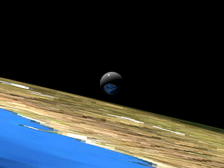
This shows how an earth model can be added to a DIRSIG scene in order to provide additional illumination on to a space-based target. An earth-sized sphere is placed in the scene and then attributed using a reflectance map derived from NASA "Blue Marble" data. When imaging a space-based object, this earth geometry will cause additional illumination in the form of "earth shine".
Earthshine Scenario
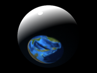
This demo simulations "earth shine" or the reflection of the Earth is a space-based object. In this case a reflective sphere has been placed above the Earth. This DIRSIG simulation models the earth via the EarthGrid plugin.
Light Curve Collection
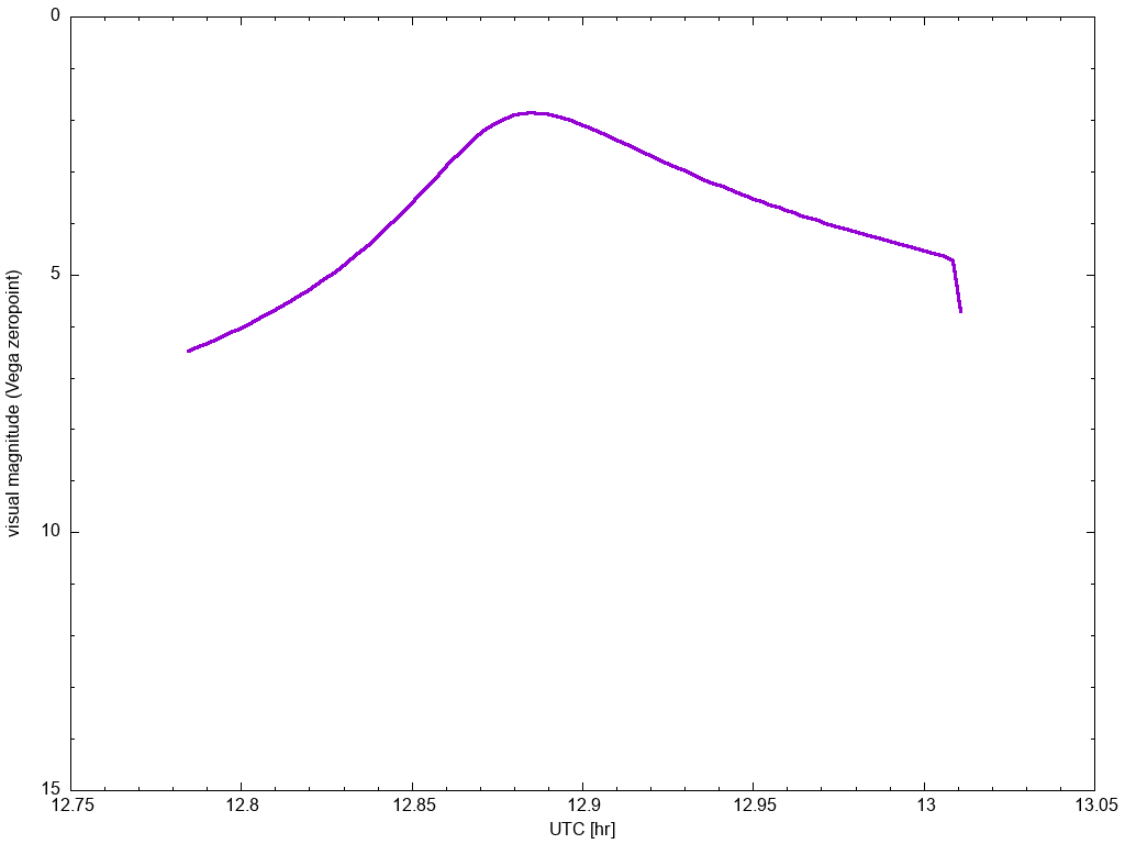
This demo shows how to use the LightCurve sensor plugin to generate a 1D (magnitude vs. time) light curve from a terrestrial observation location of a simple spherical object in orbit. The light curve captures the changing magnitude of the total reflected (and emitted) light from the object as it traverses the sky. In addition to the traditional 1D curve output, this demo describes how to use the plugin to produce a 2D "spectral waterfall" (spectral magbitude vs. time) product as well.
Space to Space Tracking Scenario
This shows how to configure a scenario with a geosynchronous satellite tracking a Low Earth Orbit (LEO) satellite. Each of the satellite orbits is specified using it’s respective Two-Line Element (TLE).
Synthetic Aperture Radar (SAR)
Please note that using DIRSIG for SAR applications is still experimental. Please consult the Radar Modality Handbook for more information about current features and limitations.
Stripmap collection of Corner Reflector Array
This demo includes a basic stripmap SAR platform configuration that collects an array of corner (trihedral) reflectors. The complex phase history file produced by DIRSIG can be focused by the supplied Matlab program to produce the final SAR image.
Spotlight collection of Corner Reflector Array
This demo includes a basic stripmap SAR platform configuration that collects an array of corner (trihedral) reflectors. The complex phase history file produced by DIRSIG can be focused by the supplied Matlab program to produce the final SAR image.
