Blackadar Plume Model

The DIRSIG Blackadar plume model is an enhanced implementation of the Monte-Carlo smoke plume model described in the book "Turbulence and Diffusion in the Atmosphere" by Alfred K. Blackadar. In Appendix E, Blackadar describes "A Monte Carlo Smoke Plume Simulation" and the book includes a simple program written in BASIC that can model a smoke plume as a series of particles that are released and perform a "drunkards walk". All equations and some descriptive text included in this document have been derived or extracted from Blackadar’s book and are noted with references. Blackadar’s published BASIC code is the basis for the enhanced C++ implementation manifested in the blackadar utility included in DIRSIG. The primary addition in our enchanced model to Blackadar’s particle (zero volume) approach is that we are modeling puffs (non-zero volume).

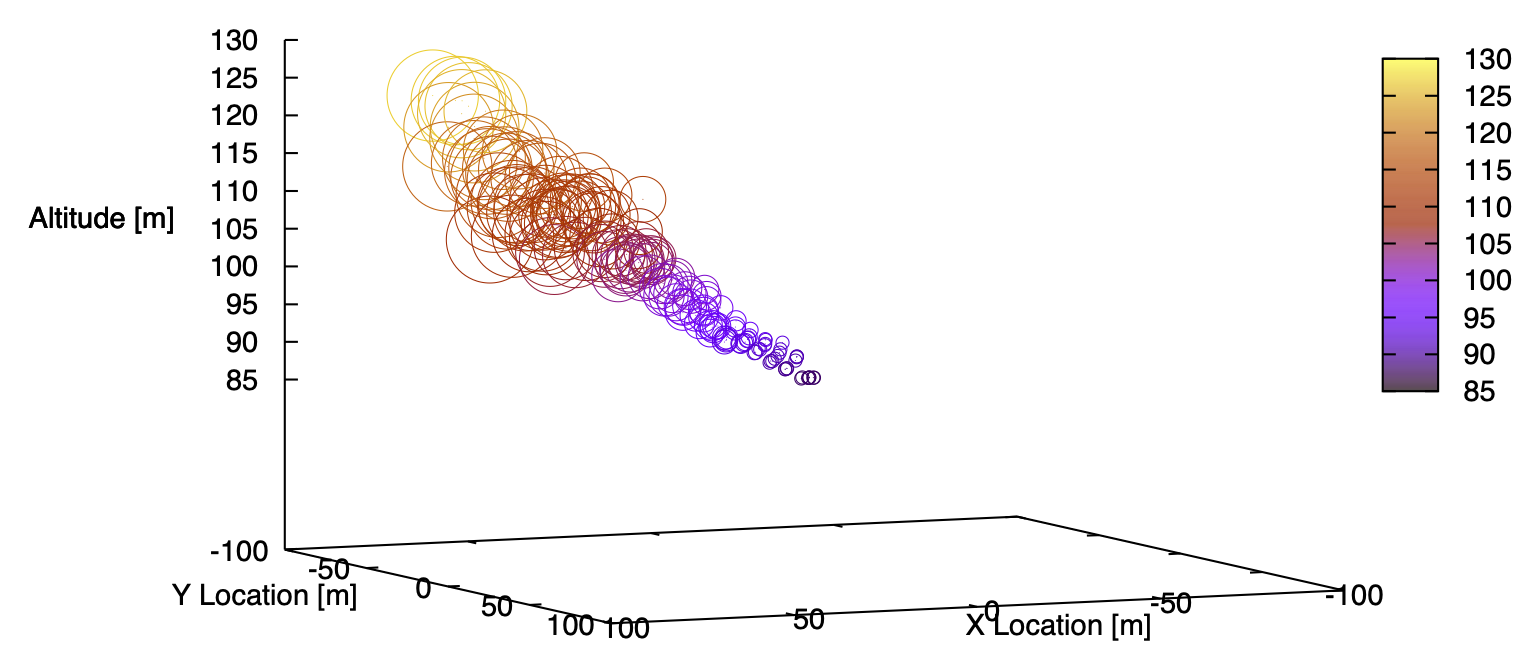
Each puff is a sphere that starts out with a specific diameter. The motion of each puff uses the same particle motion that was described by Blackadar. However, as the puff travels dispersion (from turbulence in the atmosphere) causes the puff to expand in volume. The rate of expansion is driven by dispersion coefficients which are usually different in the lateral and vertical directions. For the time being, the lateral and vertical dispersion coefficients are equal and the vertical dispersion coefficient is computed as a function of downwind range and the atmospheric stability.

When we model a turbulent wind field, there are two perspectives to consider. The first is the Eulerian perspective where we look at the statistics of the wind flow at a specific location. In the presence of a turbulent wind field, we expect the wind velocity to vary at a specific location. The second is the Lagrangian perspective where we look at the statistics of the wind field acting upon a point (particle) that moves with the flow. In the presence of a turbulent wind field, a particle traveling in that field will experience varying wind velocities as a function of time and, hence, location. In this model, we must consider an Eulerian modeling approach to describe the variation of the wind field at the stack and a Lagrangian modeling approach to describe the variation within the wind field as each particle/puff travels downwind.

As it was described earlier, the puff motion can be described as a "drunkards walk" which is described by traditional Lagrangian motion. A "random walk" would be where a particle "chooses" a totally random direction (uncorrelated to its previous direction) at each time step. In a drunkards walk, the particle "remembers" part of its previous direction (correlated) and adds a random (uncorrelated) component to the previous direction to determine the new direction. In this treatment, the puff velocity for the next time step is correlated to the current time step by combining a portion of the current velocity with a random velocity component.

\begin{equation} u( t + \Delta t) = W \cdot u(t) + u_{\mathrm{random}}(t) \end{equation}

where W is a weighting factor for the portion of the current velocity component. In the context of the "drunkards walk", this weighting factor is the fraction of the previous velocity that is remembered. The rate of memory loss is goverened by the Lagrangian time scale which is a function of the atmospheric stability classification; stable conditions will have the longest times scales and produce slow changes that result in the largest and longer lasting loops. Specifically, this weighting factor is defined by the Lagrangian autocorrelation function, \(R(\Delta t)\). The autocorrelation function describes the similarity as a function of time scales. For very small time scales we expect R → 1 (highly correlated) and for very long time scales we expect R → 0 (highly uncorrelated). For the X dimension, the velocity for the next time step can be written as:

\begin{equation} u_{x}( t + \Delta t) = u_{x}(t) R_{x}(\Delta t) + u_{x}'(t) \end{equation}

The random velocity component (\(u_x'(t)\)) is assumed to be Gaussian distributed with a zero mean and with a standard deviation (\(\sigma_{x}'\)) defined as:

\begin{equation} \sigma_{x}' = \sigma_{x} \sqrt{ 1 - R_{x}^2( \Delta t) } \end{equation}

Note, that the variance for the random velocity is also correlated through the inclusion of the autocorrelation function. The Lagrangian autocorrelation function, \(R(\Delta t)\) is assumed to have the following form:

\begin{equation} R_{x}( \Delta t) = \exp \left ( -\frac{\Delta t}{T_L} \right ) \end{equation}

where \(T_L\) is the Lagrangian integral time scale of the velocity. In this model, the Lagrangian integral time scale is computed directly from the stability of the atmosphere. For stable atmospheres, the time scale is long and for unstable atmospheres the time scale is short.

The blackadar utility program is used to generate voxelized plumes suitable for ingest by the PlumeVDB plugin. The plume is described by a small XML document contraining a series of variables. In DIRSIG4, this was stored inside the .scene file. In DIRSIG5, this can be stored in separate file that is provided to the stand-alone blackadar program.

The table following describes these variables.

There are several assumptions and caveats that should be considered when using this plume model.

The following is a list of future improvements to be made to the model.