Earth Model Plugins

This document describes the set of plugins that provide a background model of the "Earth".

These models are intended to provide background context for scenes (for example, a mountain range in the distance that changes the effective time of sunrise/sunset) or as a full scale simulation of the Earth itself.

The Earth Model API is still under development. The "EarthGrid" plugin is provided as an early example of what can be easily accomplished with this interface, but may be subject to change.

Earth model plugins are explicitly supplied in a JSIM file via the plugin list. There is no equivalent definition in DIRSIG4-era XML simulations.

EarthGrid Model

The "EarthGrid" plugin is an example of using the Earth model to provide visual indicators of location and size, drawn on the WGS84 ellipsoid. It sets up a system of lines at major and minor intervals around the ellipsoid based on the local latitude and longitude. Inputs to the model allow the user to dictate the size and color of the lines (using a simple built in 24-bit RGB mechanism).

The number of major lines is described by how many lines fall within 360 degrees, so a count of 72 would draw lines at every 5 [deg] and 21,600 at every arcminute. Minor lines are defined in the same way, but relative to the major line delta, i.e. a count of 5 would partition each 5 [deg] major line spacing into single degree interval and 60 minor lines for the arcminute setup would give arcseconds (shown below).

By default, the grid is drawn over the background color (white [255,255,255] by default). However, the user can change this color or provide a background image instead (a 24-bit RGB image)

The following example sets up a set of arcminute and arcsecond lines over a bright background:

  "plugin_list": [
    ...
    {
      "name" : "EarthGrid",
      "inputs" : {
         "major_lines" : [21600,0.00004,0,0,0],
         "minor_lines" : [60,0.00001,50,50,50],
         "background_color"  : [255,255,255],
         "altitude" : 0
      }
    },
    ...
  }

This type of setup can serve as the background of a scene, such as the Foxbat scene:

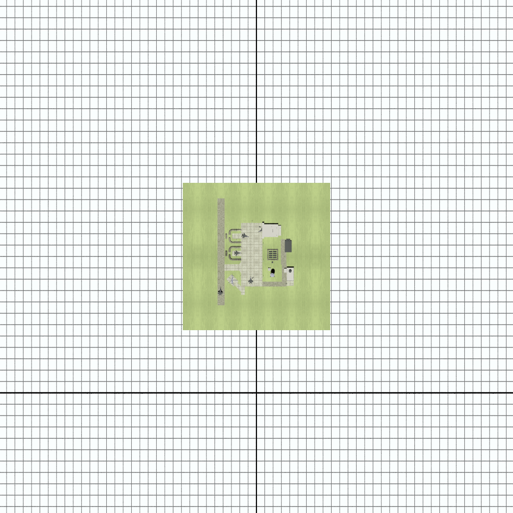
Figure 1. Using the grid Earth model to provide a background for a version of the Foxbat scene.

The tie point of the scene is 43.12 (lat) and -78.45 (lon) in decimal degrees, or 43 7' 12" and -78 27' 0" in degrees, minutes and seconds (which can be confirmed, relatively, by the major/minor lines in the image).

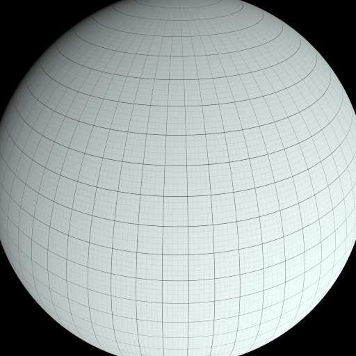
A grid might also be used in a visualization of an object in orbit — in which case, the grid would be much coarser, such as the 5 [deg] and 1 [deg] grid shown below:

Figure 2. Using the grid Earth model to provide a full Earth model.

The Earth model is not affected indirectly by scenes within the simulation, i.e. grid lines will not be shadowed by a scene and will always be visible if they are illuminated by the sun. Additionally, only rays that miss defined scenes will ever be tested for intersection with the Earth model so it is possible to have a scene that is below the Earth model and not worry about it obstructing the geometry of the scene.

The exact behavior of the Earth model will likely be covered by plugin options in the future to allow for different types of usage.

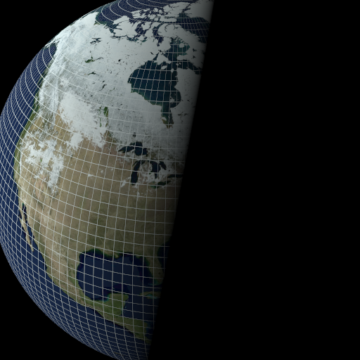
Sun shadowing can be visualized on the Earth ellipsoid based on the current Sun/Earth geometry. Using a NASA "blue marble" image:

  "plugin_list": [
    ...
    {
      "name" : "EarthGrid",
      "inputs" : {
          "background_filename" : "bluemarble.jpg",
          "major_lines" : [180,0.04,255,255,255],
          "minor_lines" : [10,0.000,255,255,255],
          "altitude" : 0
      }
    ...
  }

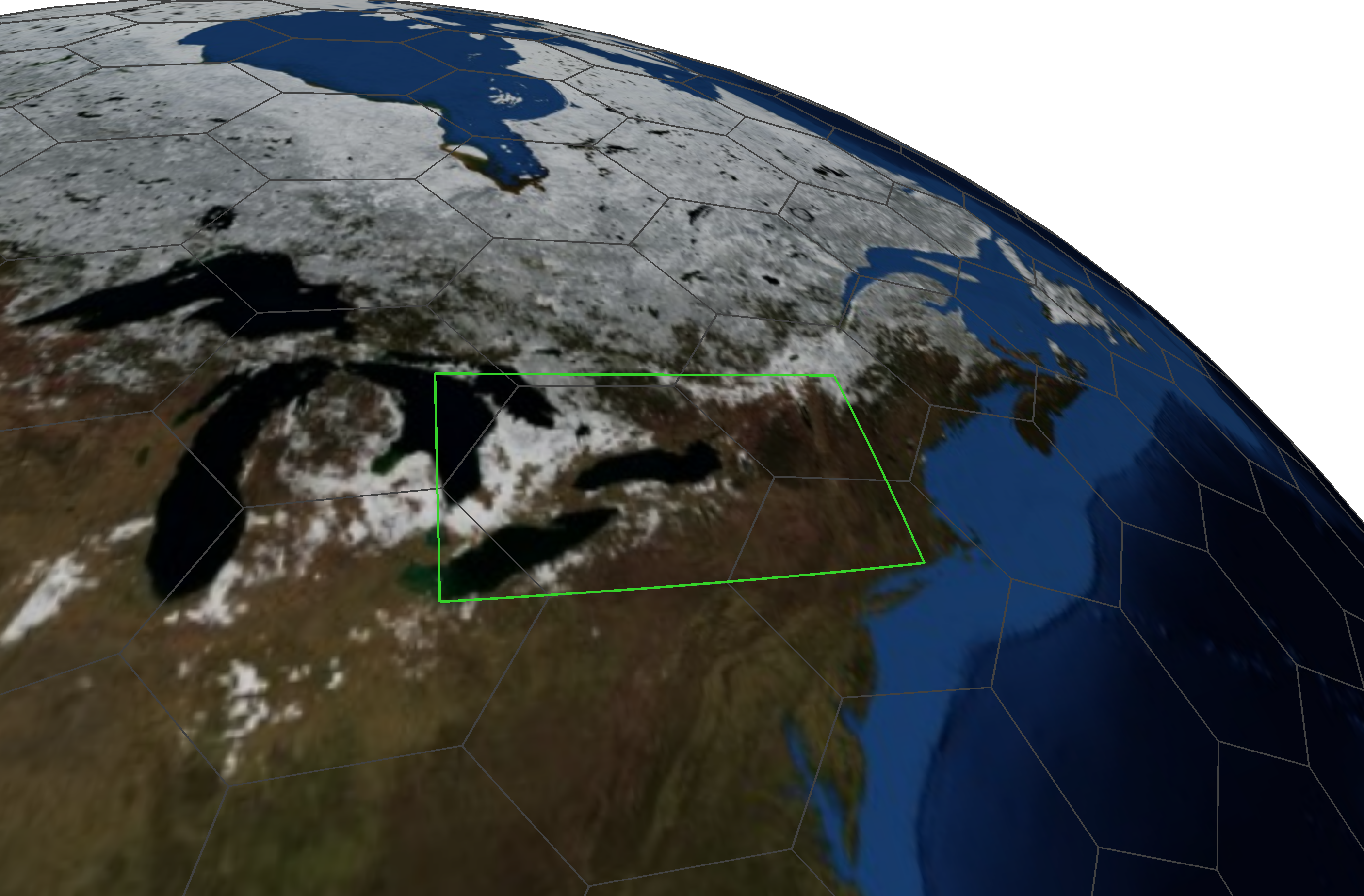
Figure 3. Full Earth model using a NASA blue marble image as the background and visualizing sunset in Rochester, NY in September.

It’s not always possible (or desirable) to provide a map for the entire Earth when focusing in on a specific region. For those cases, it’s possible to provide a latitude/longitude "box" in which the background image can be stretched (ideally when the imagery has a matching georeferenced extent).

The specific options and their defaults are listed below:

Table 1. EarthGrid Options
Name	Description	Default
`background_filename`	background image filename (24-bit RGB)	"" (empty)
`latlon_bounds`	lower-left, upper-right latitude/longitude [deg] bounds [lat0,lon0,lat1,lon1]	"" (full global coverage)
`major_lines`	definition of the major lines [count in circle, half width [deg], R,G,B]	`[360, 0.04, 0, 0, 0]` (black)
`minor_lines`	definition of the major lines [count in major, half width [deg], R,G,B]	`[60, 0.0, 0, 0, 0]` (empty)
`background`	color of the background if no image was provided [R,G,B] (all 0-255)	`[255,255,255]` (white)
`altitude`	altitude [m] of the hemisphere only visible in range: [-431:8848] [m]	`0` (sea level)

Setting the half width to 0 will avoid drawing the grid lines, which is sometimes useful when combined with the background_image option.

EarthCyclic Model

The "EarthCyclic" plugin is designed to provide true cyclic boundary conditions that account for the curvature of the Earth. Cyclic conditions are often desireable in scattering scenarios where we expect the area surrounding a "scene" to have similar scattering conditions. In essence, we want to be able to replicate the scene indefinitely in any direction to create a scattering environment that does isn’t empty space.

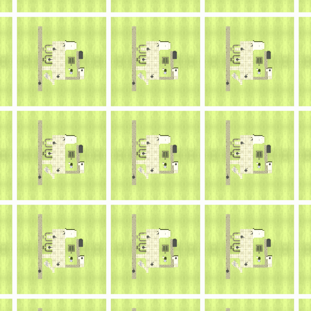
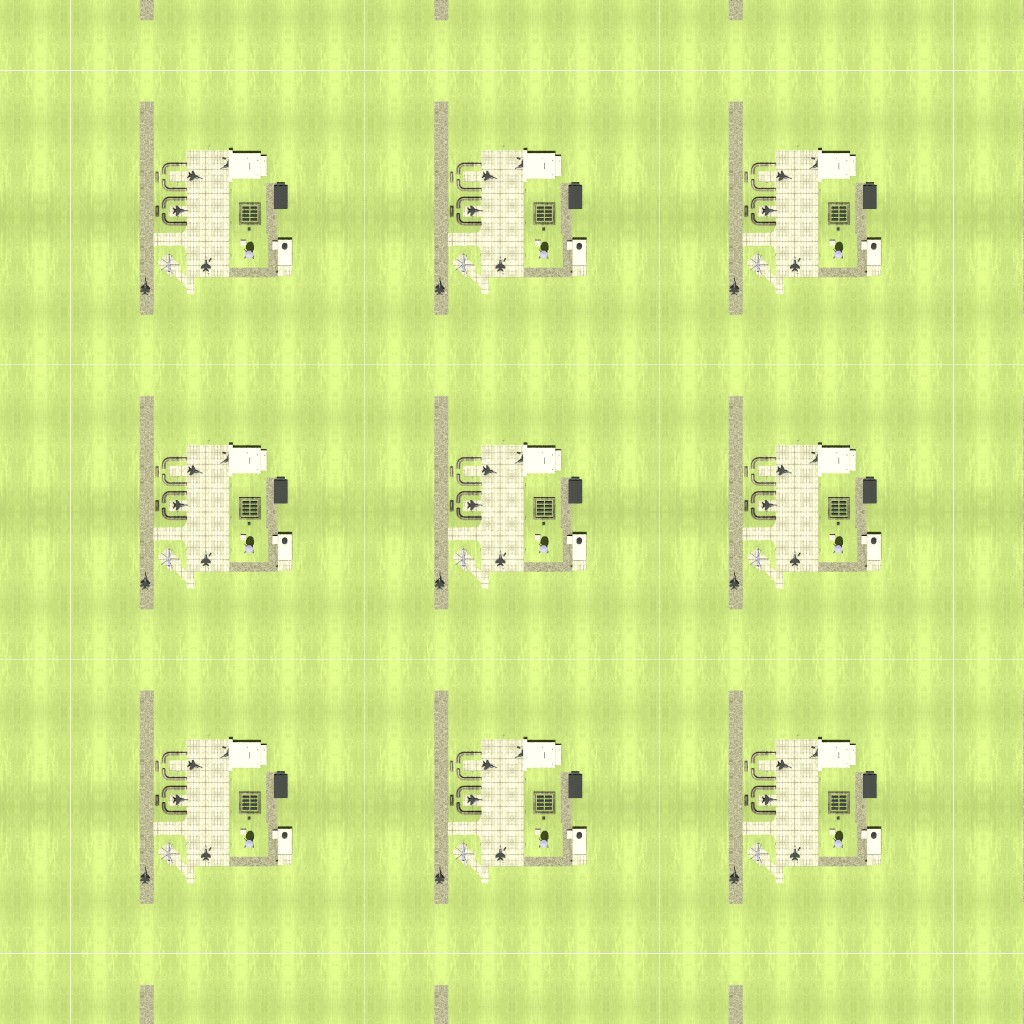
One of the common solutions to this problem is to place a "scene" in a geometry list (glist) and to then instance that scene multiple times in a grid (3x3,5x5,etc..). This is effective, but has some significant limitations. First, because of the way hierarchical instancing is handled in DIRSIG5, each scene copy may come at a non-trivial cost in terms of memory. Second, unless careful attention is paid to the translation and rotation of the scene copies, they are expanded in a tangential plane that begins to deviate from true Earth curvature as the distance increases.

The "EarthCyclic" plugin solves these problems by skipping the instancing mechanisms and translating rays over geodesic (ellipsoidal) paths to be re-traced against the original scene. It makes sure that all possible replications of the scene are tested against .. allowing slanted or horizontal paths to pass through all possible intervening scene boundaries. This process is kept somewhat efficient by the curvature of the Earth itself — rays following a straight line will eventually either diverge from the scene "horizon" or will strik a scene in a limited number of traversals.

The following example sets up cyclic boundary conditions based on the first user scene (index is zero):

  "plugin_list": [
    ...
    {
        "name" : "EarthCyclic",
        "inputs" : {
          "scene_index" : 0
        }
    },
    ...
  }

While the setup is very straighforward, the scene itself must be taken into consideration. The cylic boundary conditions are based on the bounding box of the scene (which forms the effective "tile" size of the replicated area). By default, a scene’s geometric bounding box is slightly padded to allow for some flexibility in areas in the direct vicinity of the scene (i.e. in terms of determining what needs to be handled with "global" rays versus much less expensive "scene local" rays). An option is available for the user to control this horizontal padding (assumed equal in X/Y), for example, to remove all padding, the inputs are:

  ....
  "scene_list" : [
      { "inputs" : "./my.scene", "padding" : 0 }
  ],
  ...

where the value of the padding is in units of meters. The padding can also be set to a negative value in order to trim the scene.

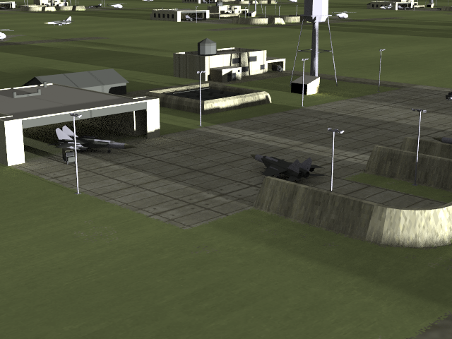
The effect of the padding can be seen using the classic "foxbat" scene as an example:

Figure 4. Tiling the foxbat scene using the default padding.

Figure 5. Tiling the foxbat scene after setting the padding to zero (the remaining gap can be removed by a smalle negative padding value).

Notes

Because the cyclic Earth model just moves the ray around, there is no change in illumination conditions across the globe (i.e. the sun location is always set to the origin scene location). Despite this, it is still possible to cast shadows from one scene to the next, as shown here:

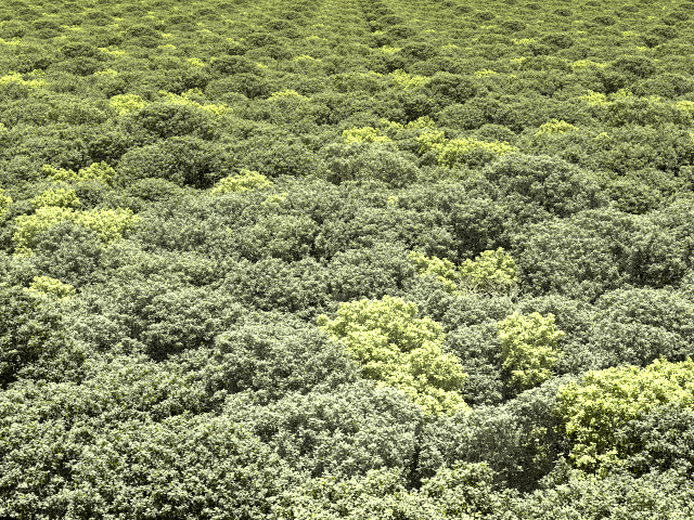
Figure 6. Slant view of the foxbat scene with cyclic conditions for a low sun. Shadows are maintained across all replicated scenes.

This continuity applies to scattering as well — radiance paths are free to propagate from one scene to the the next:

Figure 7. Slant view of a forest scene with cyclic conditions. Inter-scene scattering occurs automatically.

Cloud Model Plugins

While not part of the Earth model plugins, and in fact a separate set of plugins altogether, the cloud model plugins are closely related. They allow the user to describe clouds over very large areas, potentially over the entire globe, in the same way that the Earth model plugins allow modeling the full Earth.

FastClouds Model

The fast clouds model plugin is an analog to the simple approach to modeling clouds taken in the FastCloud2 demo. Instead of creating a reflective/transmissive cloud layer in a horizontal plane over a smaller scene, the fast clouds plugin allows the user to to define a similar layer over a lat/lon box (equivalent to the "latlon_bounds" option for the EarthGrid model).

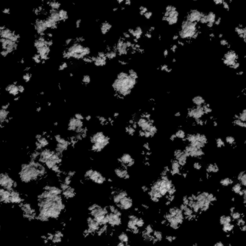
The primary input to the plugin is an 8-bit grayscale image that describes the cloud "fraction" (0-255 pixel values scaled to 0.0-1.0) and the altitude of the cloud layer [m]. During the simulation, any paths that intersect the cloud layer at the given altitude can either pass through or be reflected by the clouds (using a nominal opaque cloud spectral reflectance from Dozier (1989)). The cloud fraction is therefore both a representation of how much cloud is there and the thickness of the cloud at that point (a vast over-simplification). To account for the effect this has on the shadowing, an additional shadow "correction" is used to scale solar/lunar paths through the cloud layer (by default, it doubles the fraction — areas that already have a unit cloud fraction are unchanged).

The FastClouds model is an extreme oversimplification of cloud physics and should be used with caution. Clouds that are inherently planar (e.g. high altitude cirrus clouds) are more appropriate for the reflectance/transmission simplification, but the plugin can be used for other clouds, such as cumulous clouds with some care, especially if the signal from the cloud is expected to saturate the sensor.

Table 2. FastClouds Options
Name	Description	Default
`cloudfraction_filename`	cloud fraction image filename (8/24-bit grayscale)	"" (empty)
`latlon_bounds`	lower-left, upper-right latitude/longitude [deg] bounds [lat0,lon0,lat1,lon1]	"" (full global coverage)
`altitude`	altitude of the cloud layer [m]	"1500" (1.5km)
`shadow_correction`	fraction multiplier applied to shadow paths (up to a maximum of 1)	`2`

The following example sets up a cloud layer at 1km near the equator:

  "plugin_list": [
    ...
    {
      "name" : "FastClouds",
      "inputs" : {
          "cloudfraction_filename" : "fraction_map.png",
          "latlon_bounds" : [1.839869,26.132233,3.937533,28.179183],
          "altitude" : 1000
      }
    },
    ...
  }

Example

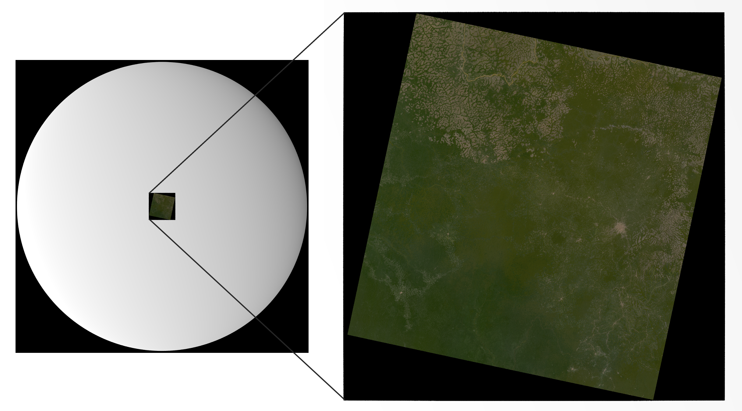
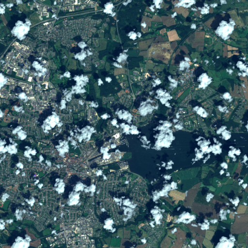
For this example, we setup a scene using the EarthGrid model and a single Landsat-9 derived image to serve as the background image (perfectly "flat" with respect to the ellipsoid with RGB properties only):

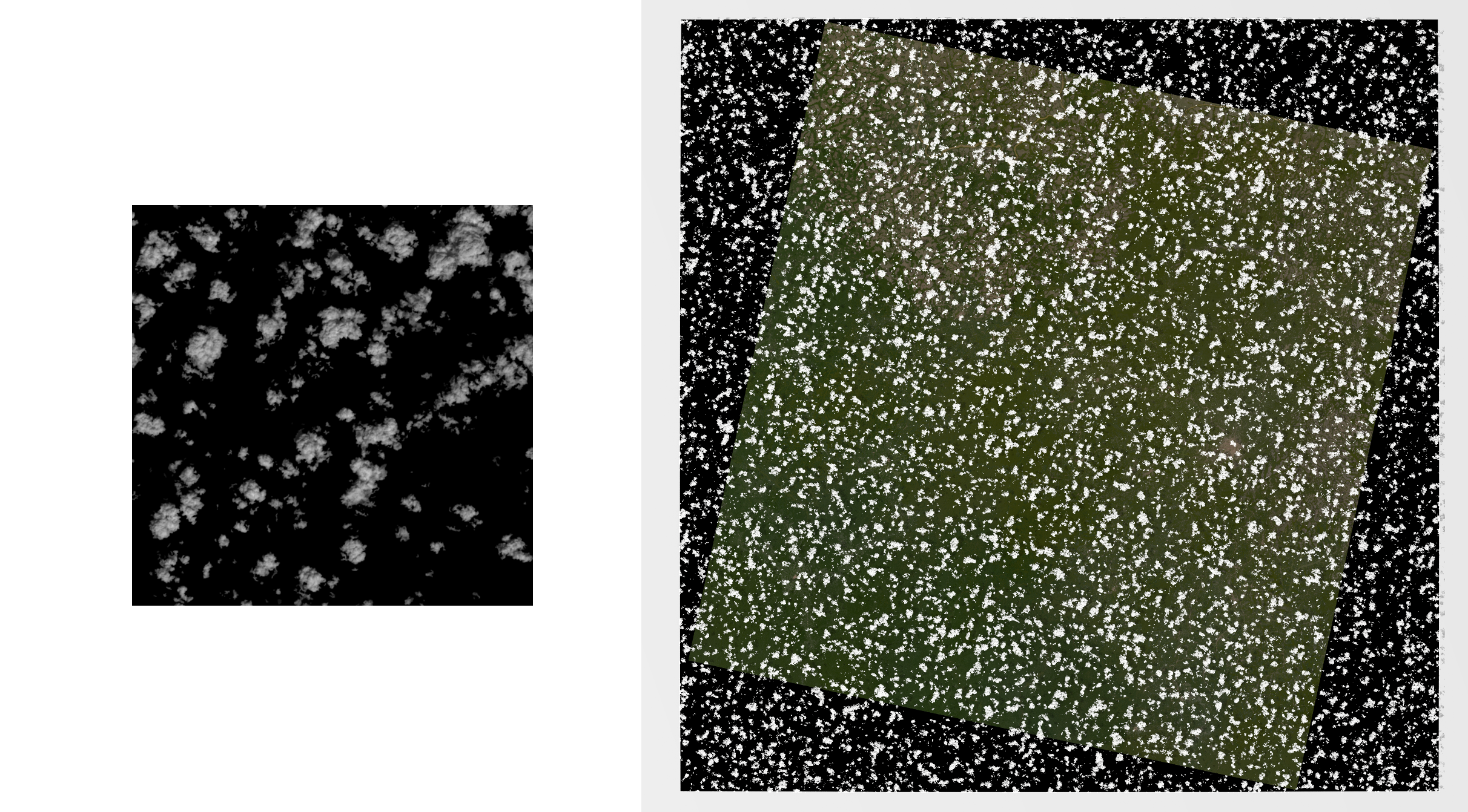
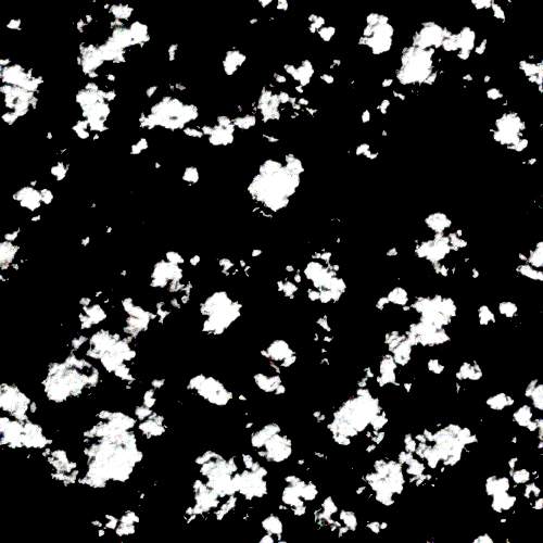
We then place a large (approximately 300km wide) cloud fraction image at 1km above the ellipsoid (as shown above). A portion of that fraction image and the full lat/lon box are shown below:

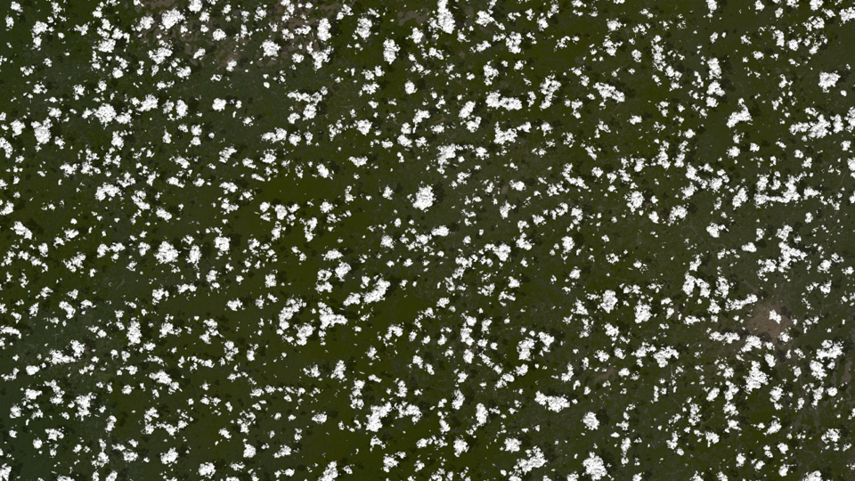
Dropping down to a more moderate resolution, we can see the cloud structure described in the fraction map coming through and the formation of shadows on the ground for a low sun angle: