The image_tool Manual

The image_tool program serves as a utility for the user to interact with the ENVI images that are output by many DIRSIG simulations.

Overview

The DIRSIG generated ENVI image files do not normally have native support in most operating systems' default image viewers, so a tool to interact with them can be useful. These images can also be viewed via QGIS or interacted with programmatically in Python via the spectral package or via GDAL. However, DIRSIG ships image_tool with the standard distribution for simplicity and to support some common operations.

image_tool is a tool-based application and operates on subcommands, similar to many other well-known CLI applications, such as git or aws. The list of available tools can be obtained via:

Example output of help tool.

$ image_tool -h
Usage: image_tool [options] <command> ...

DIRSIG Image manipulation and interaction tool

Options:
  -h/--help
	Display this help and exit.
  -v/--version
	Display build and version info and exit.
  --log_level string
	Sets the minimum logging level (debug, info, warning, error, critical, off). Defaults to info.

Commands:
  analyze
  convert
  envi
  test

For command help: image_tool <command> -h

The Convert Tool

The convert tool is used to convert ENVI images into other common image formats that can be viewed in common image viewers. This program uses QImageWriter to write output images and thus the supported output formats are determined by the abilities of that library. The reason ENVI images are output by DIRSIG is their support for arbitrary spectral bands and lossless floating point output. Since these are not features of many common image formats, this conversion will be lossy and thus has a number of options to control the conversion. For the current full list of options, use the help command, however an overview will be given here.

Usage for the convert tool.

$ image_tool convert -h
Usage: image_tool ... convert [options] filenames+

Converts ENVI format images to 8-bit RGB images for easy viewing.

NOTE:
Radiance or non-8-bit DN (digital number) images must be scaled into
the 0-255 range for viewing. This tool supports three general scaling
modes for this reason:
  * Manually gain/bias, called "manual scaling".
  * Automatically gain/bias the range [N%, (100-N)%] into 0-255, called "percent scaling".
  * Automatically gain/bias the range [μ-Nσ, μ+Nσ] into 0-255, called "sigma scaling".

NOTE:
The default behavior is '--percent 2' if no scaling options are present.

Positional Arguments:
  filenames
	The input filename(s)

Options:
  -h/--help
	Display this help and exit.
  -f/--format string
	The output file format. Defaults to PNG.
  -o/--output string
	The output filename. Defaults to input filename plus new extension.
  --stdout
	Write to stdout.
  --pixel_stride uint
	The pixel stride, to only load every nth pixel. Default is 1.
  --nan_color int int int
	An optional 0-255 RGB color to highlight NaN values.
  --zero_color int int int
	An optional 0-255 RGB color to highlight zero values.

  [Scaling]
  --gain float
	Use manual scaling, set gain.
  --gains float float float
	Use manual scaling, set gain for the R, G, and B channels separately.
  --bias float
	Use manual scaling, set bias.
  --biases float float float
	Use manual scaling, set bias for the R, G, and B channels separately.
  --minmax
	Alias for --percent 0.
  -p/--percent float
	Use percent scaling, set percentage.
  -s/--sigma float
	Use sigma scaling, set standard deviation.
  --per_band
	Apply sigma or percent scaling per-band.
  --all_same
	Apply the same scaling to all images, determined by the first image. Useful for making GIFs.
  --output_scaling
	Print scaling gains/biases to stderr.
  --autoscale string
	Supports old autoscale mode (none, percent, minmax, bandminmax, twosigma, gamma), but issues a deprecation warning. For backward compatibility only!

  [Processing]
  -b/--bands int int int
	The bands to use for RGB output. Defaults to 0, 1, 2.
  -B/--band int
	The band to use for Grayscale output.
  -x/--xyztorgb
	Convert XYZ to RGB?
  -y/--gamma float
	Set the gamma. Note: This is a gamma correction, so each pixel value is raised to 1/γ. Defaults to 1.
  -t/--tonemap string
	Set the tonemap operator: none, srgb, exp, reinhard.

The conversion can be thought of as a multi-step process:

Determine which band(s) from the input will be converted,
Determine the min and max values in the input data to be used with a linear scaling approach (discussed below in the scaling options section), and
Optionally modify the default linear scaling to a non-linear scaling approach (discussed below in the processing options section).

Band and Pixel Selection

If the --band option is provided, then a grayscale image will be produced. If the input only has a single band, then this band will be used to produce the grayscale image (e.g., the same as explicitly using --band=0).

The --bands options are used to specify which band or bands are to be mapped to the red, green and blue channels in the output image. The values provided to this option are the 0-based indices of the bands mapped to the red, green and blue channels, respectively. If the input image only has 3 bands, then the default is to assume they are in R, G, B order (e.g., the same as explicitly using --bands=0,1,2).

If the default bands variable is set in an ENVI image header file, these bands will be used as default if neither the --band or --bands options are provided.

The --pixel_stride option is used to sample which pixels will be extracted. This option can be used to downsample the image by skipping over pixels. The default stride is 1, which is to extract a pixel, move forward 1 pixel, extract a pixel, etc. Using a stride of 2 effectively downsamples the image by a factor of 2. Note that this sampling is performed in both the X and Y (row and column) dimensions of the image.

Scaling Options

The primary operation in the conversion is the scaling of floating-point data into 8-bit, integer values. Although many scaling options and combinations are available, under the hood the convert tool supports three, primary scaling methods:

Linear scaling to the range [N% → (100-N)%] into 0 → 255 using automatically computed gain and bias values, referred to as percent scaling.
- This method is available via the --percent option, where the user provides the value of N (e.g., --percent=5 will set the min and max to 5% and 95%, respectively).
Linear scaling to the range [μ-Nσ → μ+Nσ] into 0 → 255 using automatically computed gain and bias values, referred to as sigma scaling.
- This method is available via the --sigma option, where the user provides the value of N (e.g., --sigma=2 will set the min and max to -2σ and +2σ, respectively).
Linear scaling via user-supplied gain and bias values, referred to as manual scaling.
- This method is available by providing the --gains and --biases (or --gain and --bias for a single-band image) options.

Processing Options

Gamma correction

The --gamma option allows the user to apply a standard, non-linear Gamma Correction. Each value is raised to 1/γ, where γ is the the gamma value provided. This is the default processing option, with the gamma value set to 1 (e.g., the same as explicitly using --gamma=1).

Tristimulous mapping

If the input image was created with a sensor using the CIE RGB Color Matching Responses (also referred to as the "CIE tristimulous curves"), then this mapping (requested using the --xyztorgb option) will appropriately map the channel values to RGB values in the output.

Tone mapping

The --tonemap option applies a tone-mapping operation after the image has been scaled to the 8-bit range (0-255). The initial scaling is done in floating point space and this tone mapping is applied in a 0-1 floating point space and then scaled back to 0-255, so no quantization concerns should be present. See the help output for the various supported tone mappings. This option is intended primarily for making linear response images, such as radiance images, more natural-looking for visual consumption.

The following options are currently available:

none: A pass-through (linear) mapping.
srgb: Applies the standard sRGB mappings. This assumes the input image was produced using the CIE RGB Color Matching Responses.
exp: Applies an exponential mapping.
reinhard: Applies the standard Reinhard inverse-square falloff mapping (V_out = V_in / (1 + V_in))

Output Options

Output format

The --format or -f option can be used to specify the output format. The default format is the Portable Network Graphics (PNG) format (e.g., the same as explicitly providing --format=PNG). The available image format options are:

Table 1. Output format options.
Format	MIME Type	Description	Bit Depth	Platforms
BMP	`image/bmp`	Windows Bitmap	8	All
CUR	`image/x-win-bitmap`	Windows Cursor Format	8	All
HEIC/HEIF	`image/heic`	High Efficiency Image File Format	8	macOS
ICNS	`image/x-icns`	Apple Icon Format	8	macOS
ICO	`image/vnd`	Microsoft Icon Format	8	Windows
JPG/JPEG	`image/jpeg`	Joint Photographic Experts Group	8	All
JP2	`image/x-jp2`	JPEG 2000	8	Linux & macOS
PNG	`image/png`	Portable Network Graphics	8 or 16	All
PBM	`image/x-portable-bitmap`	NetPBM Portable Bitmap	8	All
PGM	`image/x-portable-graymap`	NetPBM Portable Graymap	8	All
PPM	`image/x-portable-pixmap`	NetPBM Portable Pixmap	8	All
TIF/TIFF	`image/tiff`	Tag Image File Format	8 or 16	All
WBMP	`image/vnd.wap.wbmp`	Wireless Bitmap Format	8	All
WEBP	`image/webp`	Google Web Image Format	8	All
XBM	`image/x-xbitmap`	X11 Bitmap	8	All
XPM	`image/x-xpixmap`	X11 Pixmap	8	All

The --format option will accept any of the above 3-letter format abbreviations (case insensitive). It will also accept the 4-letter JPEG and TIFF abbreviations.

All these formats default to 8-bits per pixel for grayscale or 24-bits per pixel for RGB.

For grayscale output, the user can also specify PNG16 or TIF16, which will output a single-band, 16-bit PNG or TIFF file, respectively.

Output filename

By default, the output filename is the input filename with the file format extension (e.g., .png, .jpg, etc.) appended to it (e.g., demo.img.png is produced when demo.img is the input). The --output_filename option allows the user to specify the name of the output image file.

The --output_filename option cannot be used when converting multiple images or with the --stdout option.

Output to stdout

If --stdout is specified, which will write the output file to stdout, which allows the use of shell pipes to redirect the output to another program.

Helpful Options

Scaling bands independently

The default for the automatic scaling methods (percent and sigma) is to compute a single gain and bias across all the bands, as if they were part of the same dataset. In some cases, you might want these scaling methods to compute a specific gain and bias for each band. For that use case, the --per_band option can be used.

Scaling multiple images at once

When automatically scaling a set of images in a single execution, it is useful to "lock" the scaling across all the images to avoid any image to image flicker that will arise from differences in the values (e.g., minimum, maximum, mean, etc.) in each image. The --all_same option will compute the gain and bias for the first image in the set, and then apply that same gain and bias to all the images. A common use case is making a diurnal video, where the magnitude of the images is changing during the day. If you want each frame in the video to be independently scaled, then use the automatic methods as previously described. However, if you want the scaling to be constant all day, then the --all_same option should be added. If you want to have the scaling based on the brightest image (presumably a midday image in the sequence), then provide that image as the first in the list of images.

Outputting the scaling

If you want to reveal the computed gain and bias values determined by the automatic scaling methods (e.g., percent and gamma) then specify the --output_scaling option. This is handy if you want to store the gain and bias values to apply at a later time.

Setting a color for Nan valued pixels

In some cases, the expected value of a DIRSIG pixel is NaN or "not a number". This is common in truth images to indicate that there is no value for this truth. For example, the scene_index truth is set to NaN when no scene is intersected. NaN values can also arise radiance images due to mathematical errors, including division by zero. In some cases, it is helpful to flag pixels that have NaN values by assigning them a specific color. The --nan_color option facilitates this by letting the user supply a specific RGB triplet that will be assigned to these pixels rather what the normal conversion produces. For example, the option --nan_color=255,0,0 will assign "red" to these pixels.

Setting a color for zero valued pixels

In some cases, the expected value of a DIRSIG pixel is zero. This is common in truth images with indexes such as the scene_index, instance_index, etc. to indicate that the first user scene, or instance, etc. was intersected. However, zero values can also arise radiance images when the setup isn’t correct. For example, even a surface with the reflectance set to 0 will result in a non-zero radiance if a realistic atmospheric model is used that includes path radiance arising from scattering or self-emission. In some cases, it is helpful to flag pixels that have zero values by assigning them a specific color. The --zero_color option facilitates this by letting the user supply a specific RGB triplet that will be assigned to these pixels rather what the normal conversion produces. For example, the option --zero_color=0,0,255 will assign "blue" to these pixels.

Example Usage

Converting to a color PNG image

To convert bands 16, 11 and 6 in a DIRSIG (ENVI) .img file to color PNG using a 2.5 gamma scaling, use the following example syntax:

Converting a triplet of bands into a RGB PNG image using a 2.5 gamma scaling.

$ image_tool convert --gamma=2.5 --bands=16,11,6 test.img

This will produce test.img.png since PNG is the default format.

Converting to a grayscale JPEG image

To make a grayscale JPEG file using the 1% scaling, specify the same band for all three bands:

Converting a single band into a grayscale JPEG image using a 1% scaling.

$ image_tool convert --percent=1 --format=jpeg --band=3,3,3 --output_filename=gray.jpeg test.img

or use the --band option:

$ image_tool convert --percent=1 --format=jpeg --band=3 --output_filename=gray.jpeg test.img

This will produce gray.jpeg.

Converting multiple images to color PNGs

To bulk convert a series of images, you can use standard shell wildcards on LINUX and macOS:

Converting a set of images to RGB PNGs using a 2 sigma scaling.

$ image_tool convert --sigma=2 --format=png --bands=2,1,0 demo-t0000-c*.img

This works because LINUX and macOS shells expand demo-t0000-c*.img into a list of all matching files, which is supplied to image_tool and it then iterates through that list. However on Windows, neither CMD or PowerShell expands wildcards. Instead, they simply pass them to programs and expects the program to expand them (which image_tool does not support). Hence, we need to generate the list of matches outside of image_tool and pass that list to the program. Here is an example of how to do that in PowerShell using the build-in Get-Item cmdlet:

Converting a set of images on Windows in PowerShell.

PS C:\Users\dirsig\demos\PlatformJitter1> $list = Get-Item demo-t0000-c*.img
PS C:\Users\dirsig\demos\PlatformJitter1> image_tool convert --gamma=3 --format=png $list

If you want to scale all your images the same (using the --all_same option) but the N^th image in the sequence is the one you want used to establish the scaling, then provide this image first and then use wildcards for the entire sequence. For example, supply demo-t0000-c0010.img demo-t0000-c*.img. The scaling will be established using demo-t0000-c0010.img and then applied to demo-t0000-c0000.img, demo-t0000-c0001.img … demo-t0000-c0010.img, etc. Yes, the demo-t0000-c0010.img file will be scaled twice in the process, but the simple command-line syntax is convenient.

The Analyze Tool

The analyze tool is intended to help with basic statistical analysis on images. Its full options can be seen with the help output:

Usage for the analyze tool.

$ image_tool analyze -h
Usage: image_tool ... analyze [options] operator filename

Positional Arguments:
  operator (required!)
	The analysis operator to perform.
	* extract
	  Output each band for every pixel
	* band_min_max
	  Output min/max in each band across all the pixels
	* band_mean_stddev
	  Output mean/stddev in each band across all the pixels
	* band_covariance
	  Output covariance statistics between bands
  filename (required!)
	The input filename.

Options:
  -h/--help
	Display this help and exit.
  --bands string
	The test bands. The supported formats are:
	* [band=]B
	  An individual band.
	* [bandlist=]B1,B2,...
	  An enumerated list of bands.
	* bandrange=B1,B2
	  The range of bands from B1 to B2, inclusive.
  --roi string
	The test ROI. The supported formats are:
	* pixel=X,Y
	  An individual pixel at X,Y.
	* xline=X
	  A 1D profile in X (constant X, varying Y).
	* yline=Y
	  A 1D profile in Y (constant Y, varying X).
	* rect=X1,Y1,X2,Y2
	  The rectangle from (X1,Y1) to (X2,Y2), inclusive.

Band Sampling

The --bands option is used to select which bands will be analyzed.

To select all the bands, do not include this option.
To select a single band, use --bands='band=0'.
To select a list of bands, use --bands='bandlist=0,3,4,7'
To select a range of bands, use --bands='bandrange=3,7'

Spatial Sampling

The --roi option is used select which pixels will be analyzed.

To select all the pixels, do not include this option.
To select a single pixel, use --roi='pixel=X,Y', where X and Y are the 0-based indexes (coordinates) of the pixel.
To select a vertical column of pixels, use --roi='xline=X', where X is the 0-based index (coordinate) of the column.
To select a horizontal row of pixels, use --roi='yline=Y', where Y is the 0-based index (coordinate) of the row.
To select an axis-aligned rectangular region of pixels, use --roi='rect=X1,Y1,X2,Y2', where X1, Y1, X2 and Y2 form the region from (X1,Y1) to (X2,Y2), inclusively.

Analysis Operators

The positional "operator" options define what analysis will be performed on the selected data:

To get the minimum and maximum value across all the selected pixels by band, use the band_min_max operator.
To get the mean and standard deviation across all the selected pixels by band, use the band_mean_stddev operator.
To get the covariance between bands across all the selected pixels, use the band_covariance operator.
To extract the data to an ASCII/Text, comma separated value (CSV) output, use the extract operator.

To extract the data as binary data rather than ASCII/Text, use the data tool.

Example Usage

To compute the min/max for a specific set of bands, use the following syntax:

Extracting the image wide min/max values for a list of bands.

$ image_tool analyze band_min_max --bands='bandlist=0,2,11' test.img

To compute the mean and stddev for a single band (band index = 2) within a rectangular ROI (with lower-left and upper-right image coordinates of 10,8 and 32,21, respectively), use the following syntax:

Extracting the mean and stddev of a rectangular ROI for a single band.

$ image_tool analyze band_mean_stddev --bands='band=2' --roi='rect=10,8,32,21' test.img

The Data Tool

The data tool is intended for extracting binary data from the the ENVI image file and sending it to the standard output (console, etc.). It’s primary role is as the backend for the new image viewer introduced with DIRSIG5. Its full options can be seen with the help output:

$ image_tool data -h
Usage: image_tool ... data [options] filename

Positional Arguments:
  filename (required!)
	The input filename.

Options:
  -h/--help
	Display this help and exit.
  --bands string
	The test bands. The supported formats are:
	* [band=]B
	  An individual band.
	* [bandlist=]B1,B2,...
	  An enumerated list of bands.
	* bandrange=B1,B2
	  The range of bands from B1 to B2, inclusive.
  --pixel_stride uint
	The pixel stride, to only load every nth pixel. Default is 1.

Band Sampling

The --bands option is used to select which bands will be extracted.

To select a single band, use --bands='band=0'.
To select a list of bands, use --bands='bandlist=0,3,4,7'
To select a range of bands, use --bands='bandrange=3,7'

Pixel Sampling

Example Usage

The following example extracts a single band (band index = 2) and every 3^rd pixel from the input and sends the binary data to the output.

Extracting data with simultaneous spatial and spectral sampling.

$ image_tool --bands='band=2' --pixel_stride=3 example.img
[binary data is displayable in a document]

The ENVI Tool

The envi tool is intended to provide some functionality specifically targeted to local (on disk) ENVI images. Currently, only one operation is implemented, which is a scanning of the ENVI header file to extract metadata about the image. The tool will print the requested field in the requested header file to standard output. Fields that have multiple values (curly-brace lists) will be printed with one value per line. This tool is intended for script usage to avoid potentially complicated parsing of an ENVI file with tools that are not readily available on every computing platform.

Usage for the envi tool.

$ image_tool envi -h
Usage: image_tool ... envi [options] field filename

Positional Arguments:
  field (required!)
	The header field to scan.
  filename (required!)
	The input filename (.hdr).

Options:
  -h/--help
	Display this help and exit.

Example Usage

To fetch a given ENVI header variable, you supply the field (tag) name. For example, to get the number of lines in the image file, use the following syntax:

Extracting the number of lines in the ENVI image.

$ image_tool envi 'lines' test.img.hdr
240

To get the radiometric units of the image file, use the following syntax:

Extracting the data units in the ENVI image.

$ image_tool envi 'data units' test.img.hdr
watts/(cm^2 sr um)

The quotes (i.e., '') around the field (tag) name is important when the field has a multi word name (e.g., data type, header offset, data units, etc.).

The Histogram Tool

The histogram tool is used to generate histogram data for images. Since the input images are typically high dynamic range (HDR), floating-point radiance images, there is not a predefined range and quantization for the histogram. Hence, the tool utilizes the same methods to compute min and max range as the convert tool and a user-defined option to define how many discrete bins to sort the continuous values into. Its full options can be seen with the help output:

Usage for the histogram tool.

$ image_tool histogram -h
Usage: image_tool ... histogram [options] filenames+

Computes the histogram for images.

Positional Arguments:
  filenames
	The input filename(s)

Options:
  -h/--help
	Display this help and exit.
  --stdout
	Write the hisogram data to stdout.

  [Band Selection]
  -b/--bands int int int
	The bands to generate a RGB histogram for.
  -B/--band int
	The band to generate a grayscale histogram for.

  [Range and Sampling]
  --minmax
	Alias for --percent 0.
  -p/--percent float
	Determine range using percent of values, set percentage.
  -s/--sigma float
	Determine range using mean and sigma, set standard deviation.
  --bins int
	The number of bins used for the histogram (default = 256).

Band Selection

The tool can produce the histogram for either a single band or band triplet (e.g., RGB). The --band and --bands options allow the user to select the single or multiple band generation, respectively. See the same options in the convert tool for more information.

If the default bands variable is set in an ENVI image header file, these bands will be used as default if neither the --band or --bands options are provided.

Range and Sampling

The min and max values (range) for the histogram can be computed as the absolute minimum and maximum (via the --minmax option), by excluding a percentage of the total dynamic range (via the --percent option) or as the mean +/- a used supplied number of standard deviations (via the --sigma option). To match the default of the convert tool, the default is the equivalent of --percent=2. The number of bins used to quantize the (nearly) arbitrary precision floating-point data is provided by the --bins option (the default is 256 bins).

The min and max values for the histogram are computed across all the bands selected to produce a common set of bins.

Example Usage

To generate a histogram for an RGB image (with the default bands tag set in the ENVI header file) that excludes the pixels in the top/bottom 1%, use the following syntax:

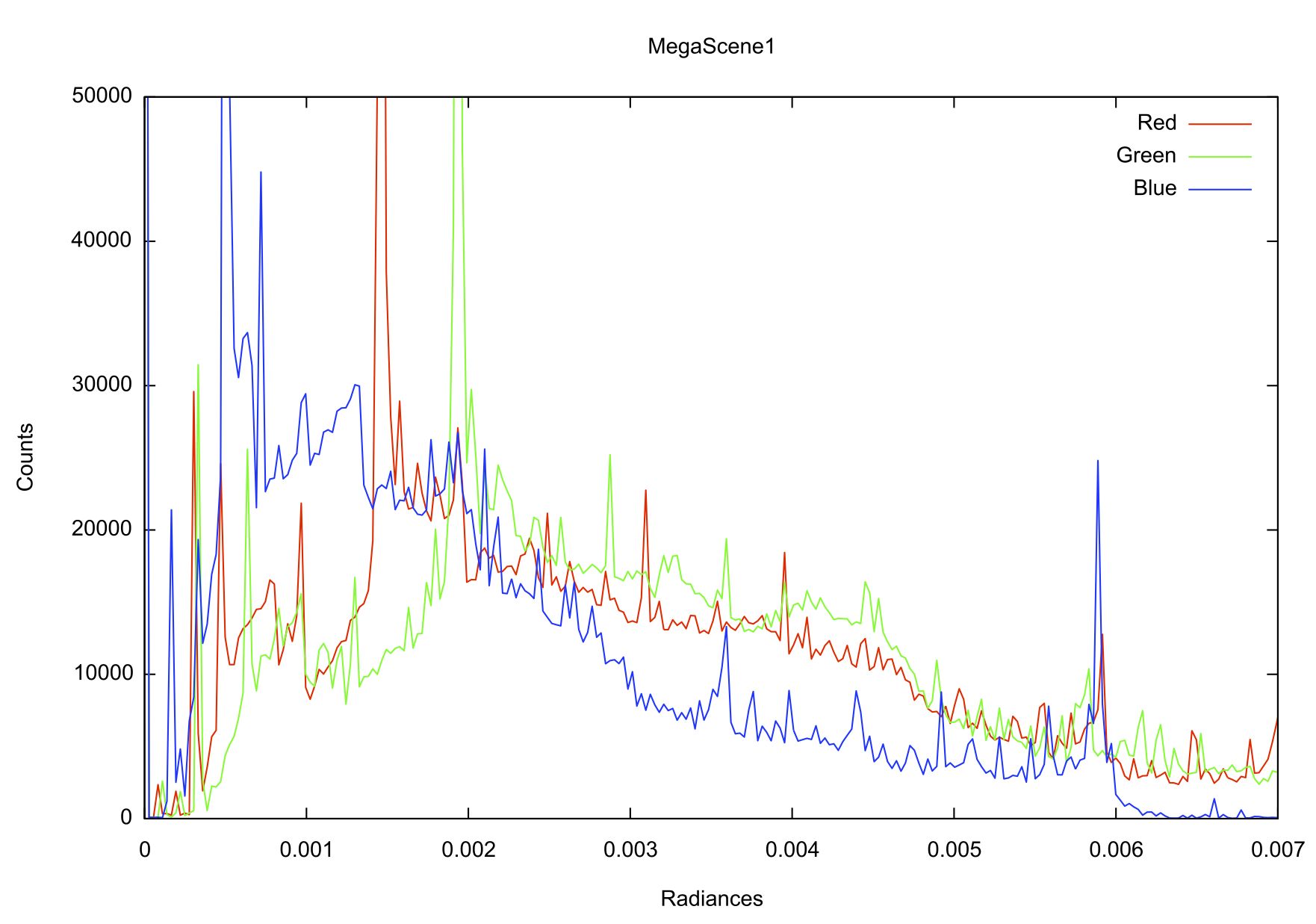
Extracting a histogram for an RGB image using the 1% range method.

$ image_tool histogram --percent=1 rgb.img

The output histogram data is an ASCII/Text file with the .txt extension appended to the input image filename (e.g., rgb.img.txt for the input rgb.img file in the example above). The first column of data is the bin index (0-based), the second column is the corresponding bin value (e.g., radiance, photons, etc. depending on the units of the input file) and the remaining columns are the number of pixels that had values for the respective bin (either 1 or 3 columns will be present depending on the band selection).

Example output histogram data file.

# Histogram data produced by 'image_tool'
0 0.00000e+00 178559 178966 180504
1 2.76459e-05 97 99 99
2 5.52919e-05 80 76 80
3 8.29378e-05 2352 88 98
4 0.000110584 348 2598 66
...
[lines deleted for documentation purposes]
...
250 0.00691148 3649 2776 87
251 0.00693913 4114 2589 69
252 0.00696678 5329 3305 88
253 0.00699442 6709 3224 71
254 0.00702207 8174 3487 99
255 0.00704971 79504 98195 41810

This data can be plotted in any 2D plotting tool, as shown below using gnuplot.

Figure 1. Plot of RGB histogram data.

The Test Tool

The test tool is used to make and perform tests on images. This can be useful for making assertions about DIRSIG output. Tests can be specified in a JSON format either via a file or through stdin with the --stdin option. An example test input is:

Test Definition

Example test JSON document

[
  {
    "filename": "rgb.img",
    "tests": [
      {
        "id": "band_mean",
        "name": "Spatially-averaged band values for the image",
        "description": "Verifies the spatially-averaged band values of the image.",
        "history": "Test automatically generated with 'image_tool' 2021.30 (04678d1)",
        "metric": "band_mean",
        "expected": [0.01513, 0.01513, 0.01513],
        "tolerance": [1.513e-05, 1.513e-05, 1.513e-05]
      }
    ]
  }
]

The structure of the JSON document is an array containing objects for each image file to be processed. Each image file object contains the filename variable with the name of the image file and a tests object that is an array of tests to be performed. Each test object contains the following:

Metadata

Each test contains a set of variables describing the test:

The id is a unique string for each test that is used to reduce duplication when running multiple tests in a single execution of the tool. These IDs must be unique within a set of tests run in a given execution.
The name is the short name for the test that is displayed when the test is run. It should contain a unique and brief but descriptive string.
The description is available to capture a more detailed description of the test. It might provide important details about the test and what it attempts to achieve.
The history is available to document the history of the test and will typically contain who made the test and when.

Metrics

The supported values for metric are:

"band_mean" → The mean of the ROI for each band
"band_min" → The minimum of each band in the ROI
"band_max" → The maximum of each band in the ROI
"band_min2" → The mean of the bottom 2% of values in the ROI for each band
"band_max2" → The mean of the top 2% of values in the ROI for each band

The expected value for the metric is supplied via the expected array. The dimension of this array is based on the number of bands (channels) in the image or the band selection defined in the test (see below).

Tolerance

The tolerance defines the allowable deviation of the computed values from the expected values. Like the expected values, this is an array sized to match the number of bands (channels) used in the test. The tolerance is in the same units as the data. Alternatively, the tolerance can be specified as percentage (via the percentage array rather than the tolerance array), where each array element is a percentage (0-100) error (from expected) that can be tolerated.

Band Subsets

By default, the metric is computed for all bands in the image. The bandSubset can be used to confine the bands over which the statistics are calculated. This field is an object of the form:

    "bandSubset" : {
      "type": "band",
      "value": [0]
    }

The supported values for type are band, list, and range.

For band, the values array contains a single band index.
For list, the values array contains arbitrary number of band indices.
For range, the values array contains a band index pair that defines the start and index (inclusive) of the band range.

Any of these band indices can also be substituted with a string of the form $<BAND_NAME:name>, where name is the name of the band in the image file. This can be especially useful when defining tests for the classic DIRSIG truth image data cube. Using the band name makes it more robust if more truth is added to the image and the band indexes change.

Example single band subset using the BANDNAME option.

    "bandSubset": {
      "type": "band",
      "value": [ "$<BAND_NAME:Dominant Material Index>" ]
    },

Spatial Subsets

By default, the metric is computed for all pixels in the image. The roi allows the test to restrict the set of pixels that the metric is computed for. This field is an object of the form:

    "roi" : {
      "type": "rect",
      "value": [0, 5, 10, 15]
    }

The supported values for type are pixel, xline, yline and rect.

For pixel, the value array should contain 2 elements indicating the X,Y coordinate of the pixel.
For xline and yline, the value array should contain a single element indicating the x or y index at which to take a line profile.
For rect, the value array should contain 4 elements indicating the min_x, min_y, max_x and max_y coordinates of the rectangular region.

Making a Min/Mean/Max Test

There is an option to the test tool to generate a simple image statistics "fingerprint" test:

Creating a simple, statistics "fingerprint" test.

$ image_tool test make demo.img > stats.json

This will compute the image min 2%, max 2% and mean values and automatically create a test to confirm them.

Using the test make combination is also a good way to generate the basic JSON document for a test that can be manually customized.

Updating an Existing Test

If you have an existing test JSON file and need to update the expected values to match an existing image, then the test update option can be used:

Updating an existing test.

$ image_tool test update truth_tests.json

Running a Tests

To run a test, the test run option should be used:

Running an existing test.

$ image_tool test run truth_tests.json

The output of the tool is a JSON document containing an object for each file processed, and each test on that file. Each test object contains the id and name for the test as well as a success variable:

JSON output of a successful test.

[
  {
    "filename": "demo_truth.img",
    "tests": [
      {
        "id": "outside_plane1a.test",
        "name": "Outside Plane, position #1, time #1",
        "success": true
      },
      {
        "id": "outside_plane1b.test",
        "name": "Outside Plane, position #2, time #1",
        "success": true
      },
      {
        "id": "inside_plane1.test",
        "name": "Inside Plane, position #2, time #1",
        "success": true
      }
    ]
  },
  ...
]

If the test fails, the success variable will be set to false and the error variable will contain a string describing which band(s) failed the test, the computed image value, the expected value and the difference.

JSON output of an unsuccessful test.

[
  {
    "filename": "demo_truth-t0000-c0000.img",
    "tests": [
      {
        "error": "Band    Image           Expected        Abs Diff        % Diff\n0       3.102620e+02    3.122620e+02    2.000000e+00    0.640488",
        "id": "tests_d5/outside_plane1a.test",
        "name": "Outside Plane, position #1, time #1",
        "success": false
      },
      ...
    ]
  }
]

Using Python-based Tests

As an alternative to the statistical tests given above, image_tool also supports running user-defined tests using Python. This can be done with slight modifications to the test JSON:

Example Python test JSON document.

[
  {
    "filename": "rgb.img",
    "tests": [
      {
        ""
        "description": "Runs a user-defined Python Test",
        "history": "Developed by <name>",
        "id": "user_defined_test_0"
        "name": "MyTest",
        "pyModule": "image_test",
        "arguments": ["15"]
      }
    ]
  }
]

This example would look for the "image_test" module in your PYTHONPATH, which would include the current working directory. Normally, this would correspond to a file called image_test.py. Additional paths may be added via the --pythonpath argument on image_tool test run. In this file, there should be a global function called test, for example:

import numpy as np

# args is present only if "arguments" is in the JSON
def test(image, args):
    exp = float(args[0])
    sum = np.sum(image)
    return abs(sum - exp) < 0.01, f"Expected sum to be {exp}, was {sum}"

The first value of the return tuple should be a boolean indicating the success of the test and the second should be an error string that will be shown upon failure. Note that "arguments" is an optional field in the JSON and should be omitted from test()'s argument list if it is not provided.