Inherent Optical Property Model (IOPModel) Plugin

Introduction

In order to use the entire water model effectively, the user will need to have a way of defining the spatial distribution and form of IOPs (inherent optical properties). This documentation addresses the definition of basic IOP models and the interface that is available through the IOPModel plugin. We take the approach of emphasizing the basic form of established models rather than focusing on specific parametrizations, so that newer data can be more easily integrated into the model without having to write new functions.

Implementation summary

The practical implementation of the IOP model was done by adding inter-related models of IOPs in DIRSIG that describe the interaction between component IOPs and interface with the rest of DIRSIG through the plugin interface. Additionally, the model handles the common spatial distribution of the physical properties of the water, e.g. the concentration of constituent components such as chlorophyll. The IOPModel plugin is defined through the usual jsim interface using a "Water" entry in the "medium_list" section (see the water_medium description for more details) and contains a single input parameter, the name of an external file describing the inputs to the model. This was done to allow quick use of previous setups in DIRSIG4 which used the same tabulated input format. An example usage of the plugin in shown below:

{
    "name" : "IOPModel",
    "inputs" : { "iop_filename" : "clear_water.iop" }
}

Within the input file is a single top level tag section called "IOP_MODEL". The IOP_MODEL is initialized by a base medium (usually pure water, but it could be air or even a null (void) medium) that defines the basic bulk properties. Additional IOPs are added by linear combination, are defined in individual models and are allowed to communicate with each other (for covariant models, for instance). Since the definition of the IOP_MODEL is associated with a particular medium in the "medium_list" it is possible to have many models tied to different volumes within the same scene which have vastly different IOPs and constituent concentrations.

The IOPModel plugin is a wrapper around all of the linear IOP models (which can contain many IOP models themselves) as well as two additional models: the aggregate concentration model and the single refractive index model. It exists primarily to enable cross talk between the various models. Thus, multiple IOP models can query a concentration model at a point to determine the local constituent concentration; an absorption coefficient model can be dependent on the results of another model; scattering phase functions can easily be linked to the appropriate scattering coefficient models. These inter-relationships are necessary in order to fully implement many of the common theoretical/empirical IOP models that exist within the literature and that represent natural waters.

Base media

Each IOP_MODEL section is initialized with a base medium that fills out the basic optical properties of the medium, though the user is able to eliminate all initialization by using the "null" base medium (the refractive index does is set to 1.0 by default). To define the base medium, the user adds a BASE_MEDIUM parameter to the IOP_MODEL section of the material file. Each additional IOP model is defined independently in its own subsection (as described in the absorption, scattering, phase function, etc… sections that follow). A typical IOP_MODEL description might look like this (with the base medium defined at top):

IOP_MODEL {
    BASE_MEDIUM = purewater
    ADD_SCATTERING_MODEL {
        ...
    }
    ADD_ABSORPTION_MODEL {
        ...
    }
    ADD_PHASE_FUNCTION_MODEL {
        ...
    }
    ADD_CONCENTRATION_MODEL {
        ...
    }
}

where the added model definitions are described later.

The null medium

As stated previously, the user may use a null base medium for the IOP model. This effectively sets the absorption and scattering coefficients to zero and the refractive index to one at all wavelengths. The scattering phase function is effectively a spherical delta function in the forward direction. In practice, the null medium does not physically exist as code. Instead, all of the initial values of the IOPs will be initialized to null values.

The air medium

The air base medium is essentially the same as the null medium, but uses a refractive index of 1.0003 instead of 1.0. Practically speaking there is very little difference between the two, but the air medium is useful for clarity.

Pure fresh water

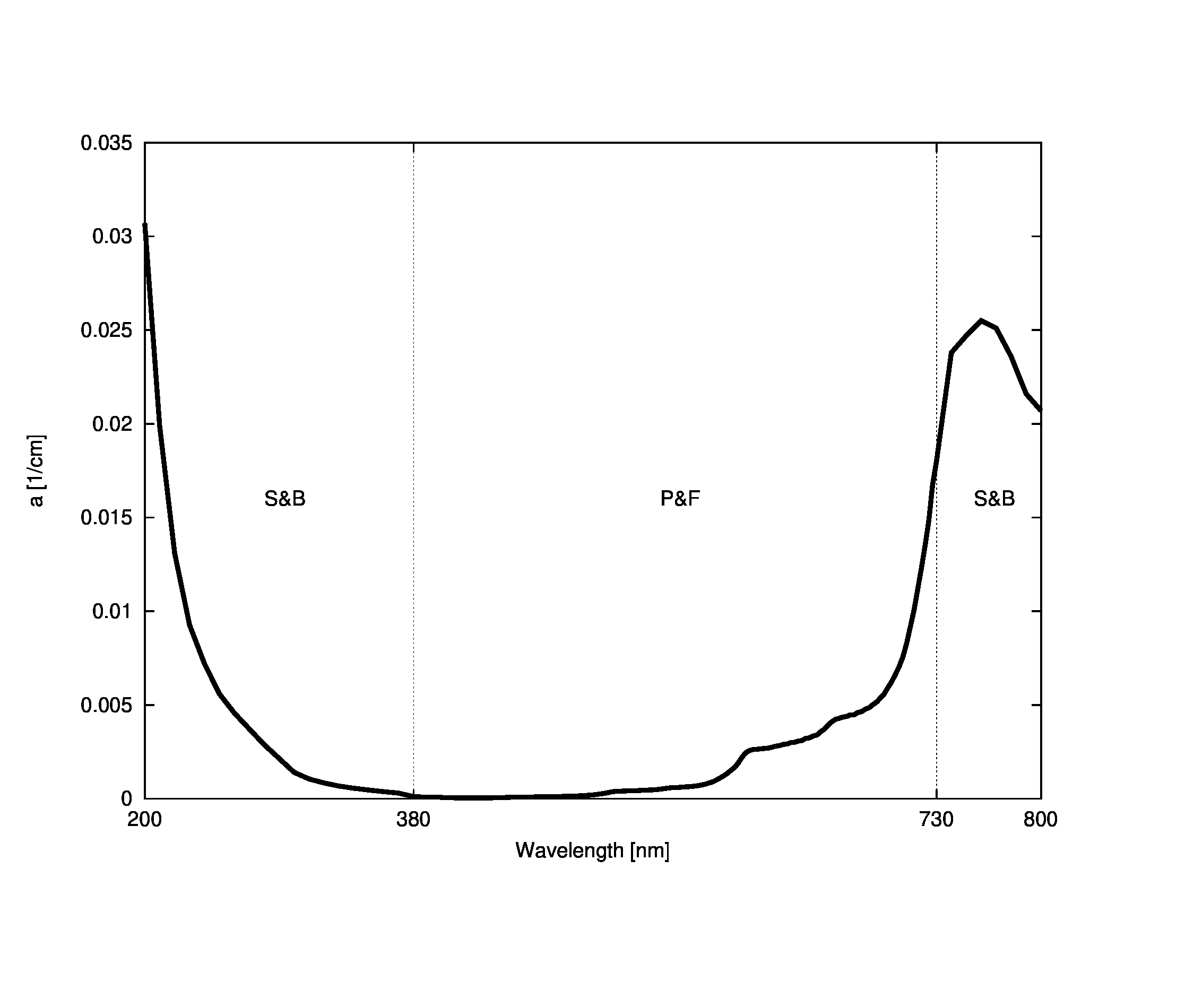
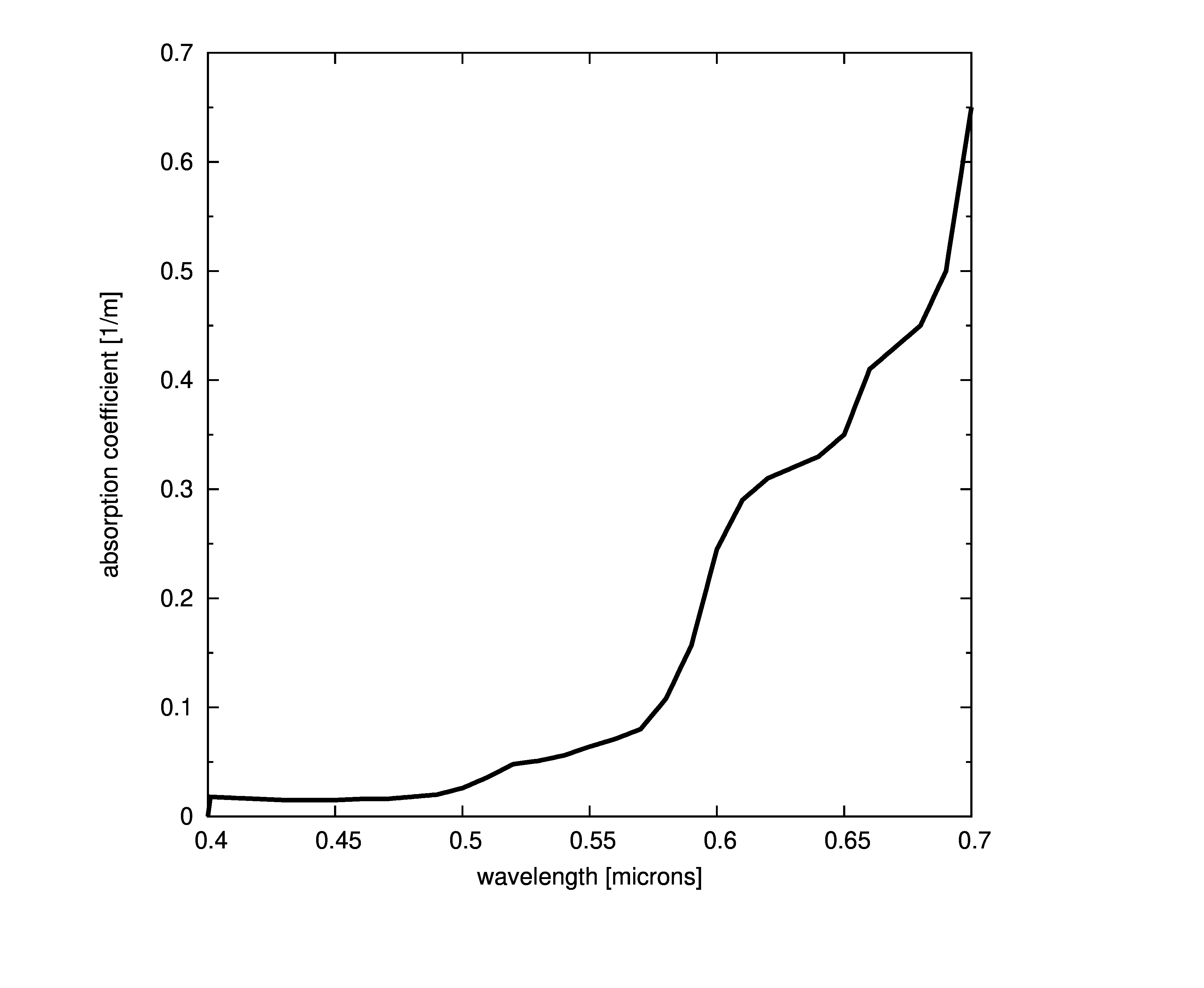
The base medium used for most water modeling runs will be a pure fresh (i.e. low salinity) water model, or purewater. The absorption coefficient is derived from two studies. The first (Pope and Fry) is more recent and provides absorption data from 380 nm to 730 nm in 2.5 nm increments. The second (Smith and Baker) is an older and more sparsely sampled source, but it provides data to extend the range from 200 nm to 800 nm (in 10 nm increments). Data for wavelengths between sampling increments are linearly interpolated. The final shape of the absorption coefficient curve is shown in the figure below with the component models marked.

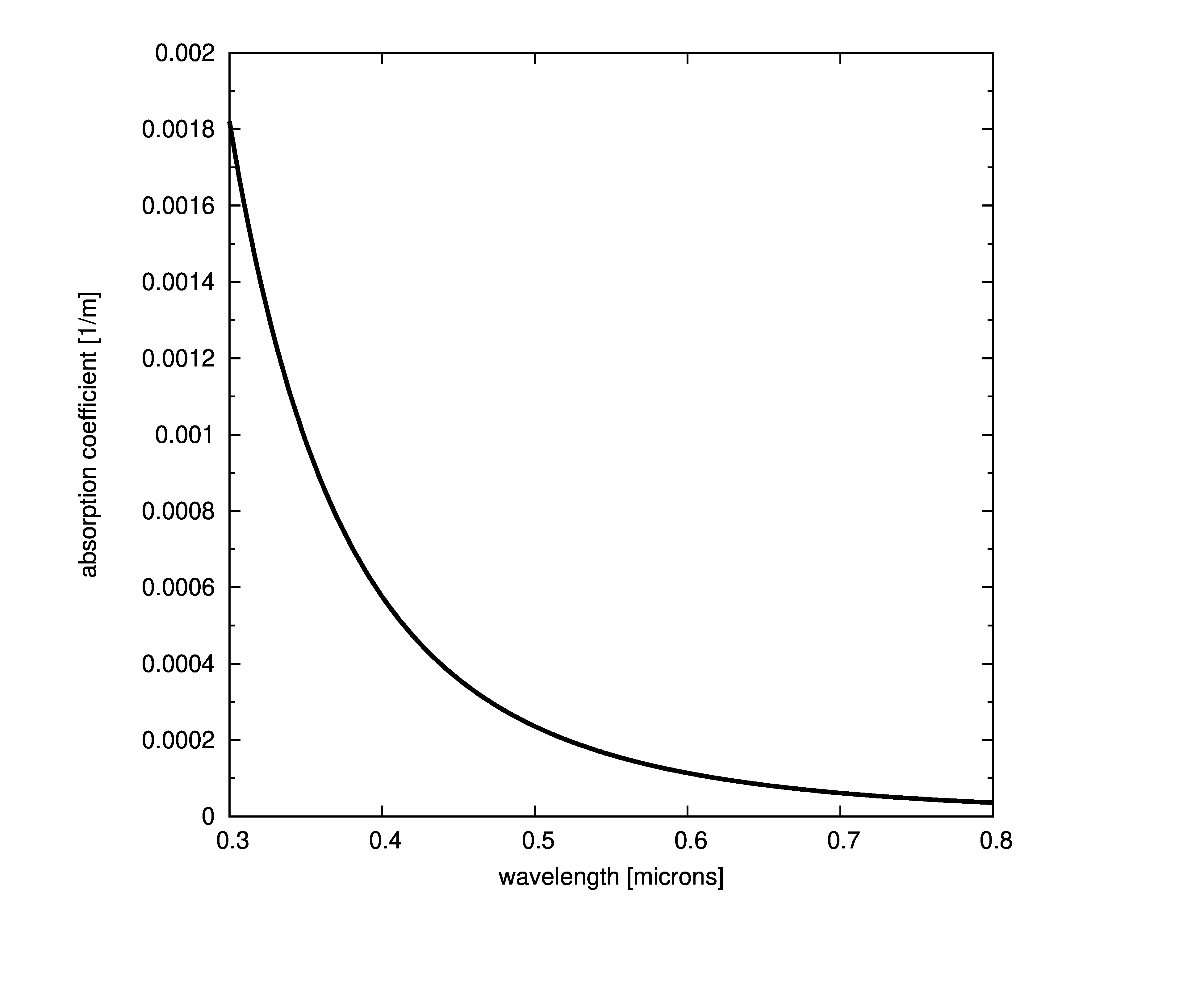
The scattering coefficients for pure water are based on . A power function was fit to the data, resulting in

\[\begin{aligned} b(\lambda)&\cong&3.4123664\cdot 10^8\lambda^{4.1537676}.\label{eq: buiteveld} \end{aligned}\]

No claim is made as to the accuracy of data obtained from this equation outside of Buitevel’s limits (340 to 750 nm), it is only provided as a guess given that the form in the measured region does appear to have an underlying power function structure. The spectral pure water scattering coefficient is shown below

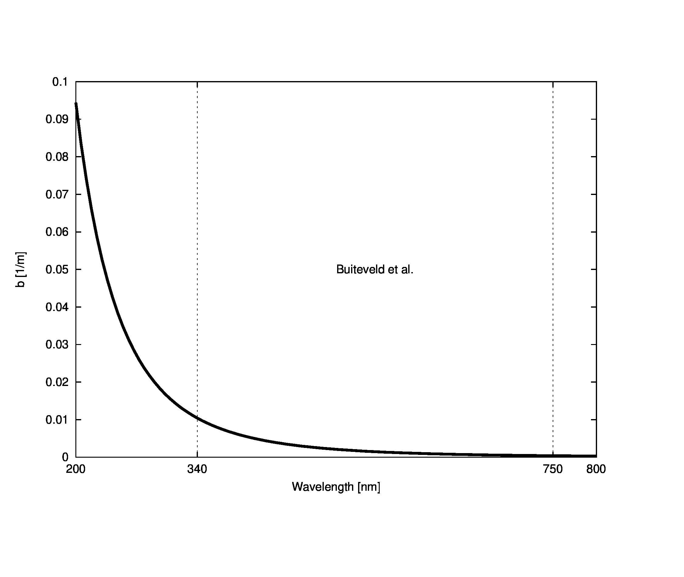
More complex data from accounts for salinity and pressure, but we will assume that Buiteveld’s data is sufficient for our purposes of modeling fairly standard fresh waters.

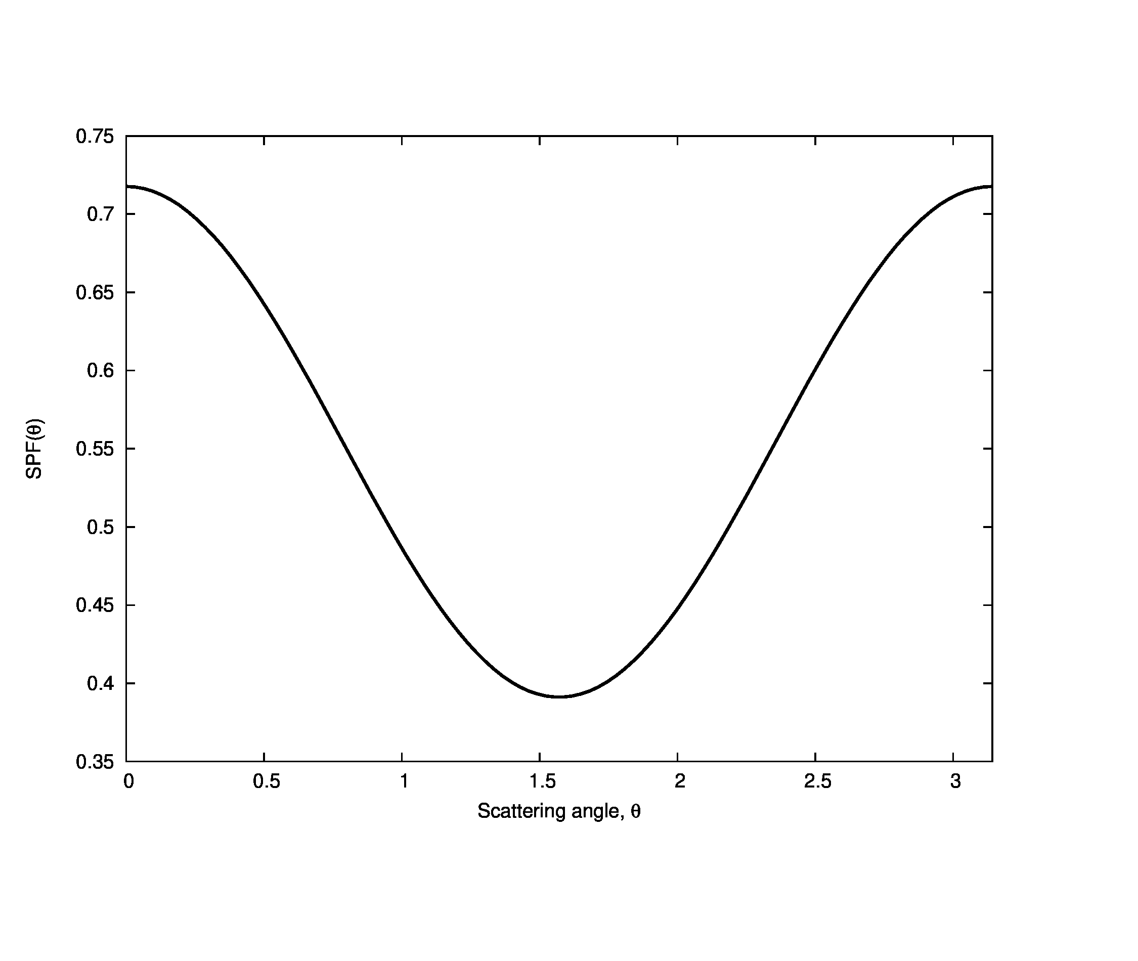
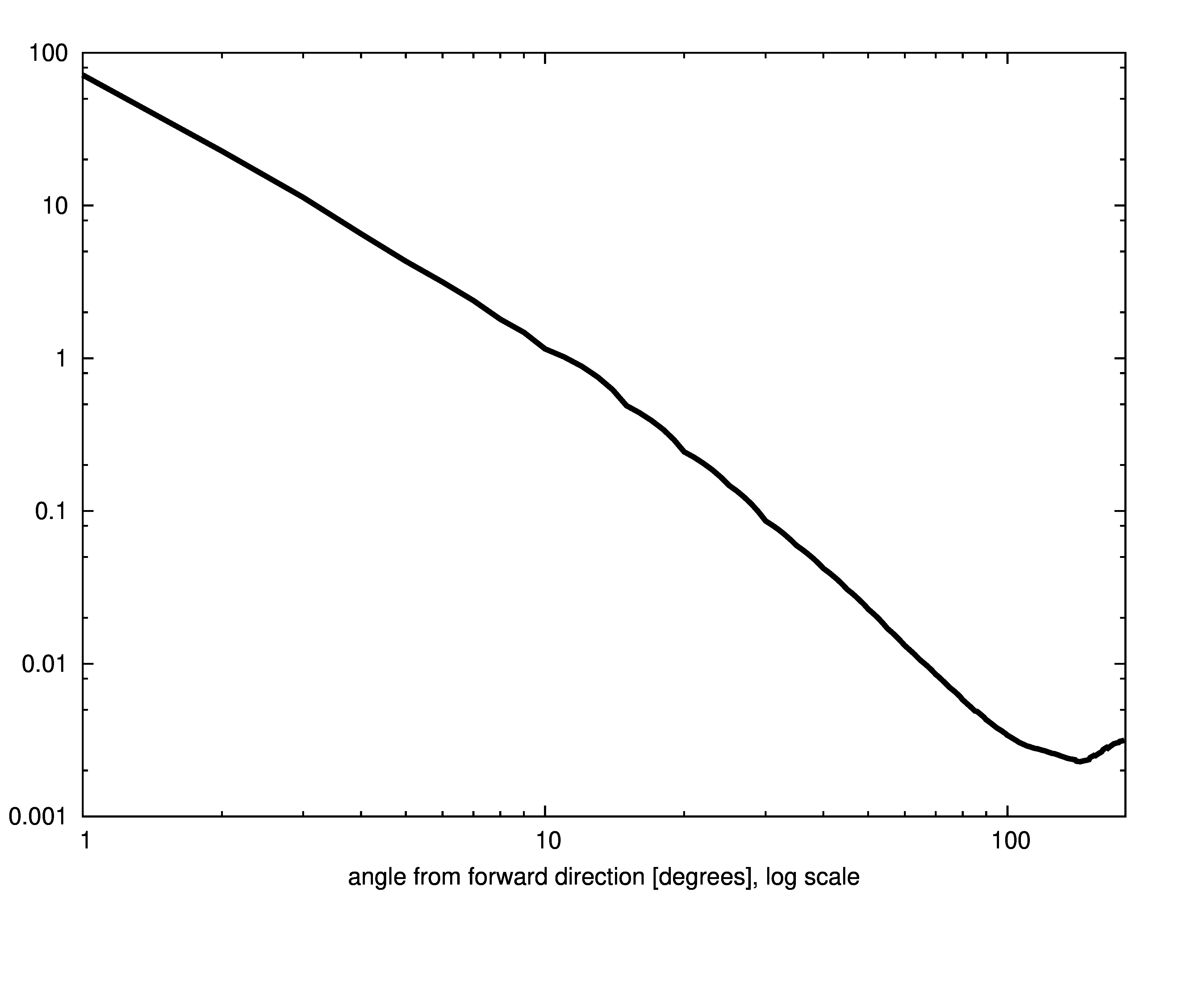
The scattering phase function for pure water has been found to have a roughly Rayleigh form,

\[\begin{aligned} \tilde{\beta}(\theta)&=&2\pi\left(0.06225(1+0.835\cos^2\theta)\right)\notag\\ &=&0.391128+0.326592\cos^2\theta\label{eq: rayleigh}, \end{aligned}\]

where \theta is the scattering angle measured from the forward direction (all of the scattering phase functions we will be using are rotationally symmetric). The shape of the phase function is shown below:

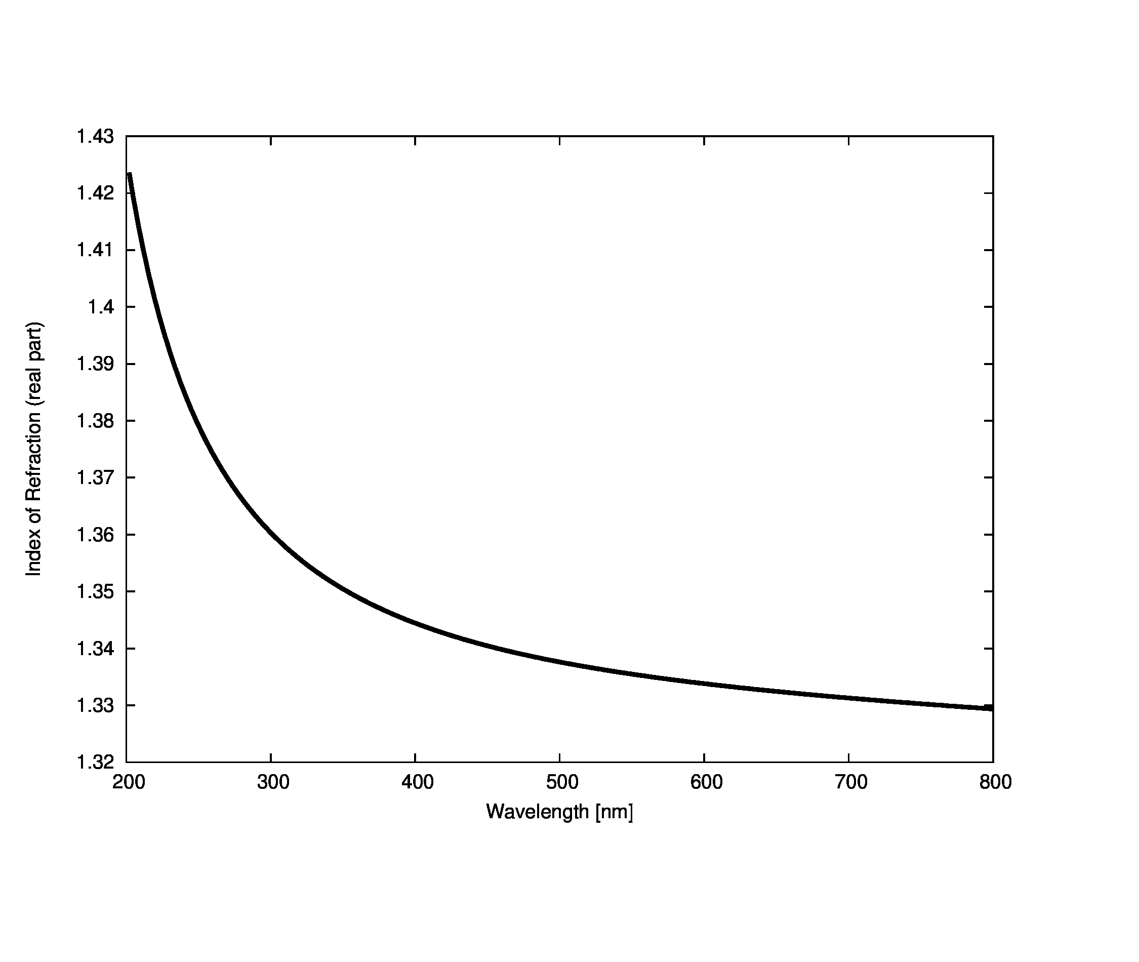
The spectral refractive index of pure water is taken from the IAPWS model . While this refractive index model is parametrized by both temperature and pressure, the effective differences are minor and will be ignored by this base model. We choose to use the curve produced by a temperature of 286 K (a mid-range value for water bodies in New York state) and a single atmosphere of pressure. The results are shown below:

Other pure water models

Besides purewater there are a number of other pure water base media that are provided that use slightly different combinations of IOPs for comparison purposes with other models. Base medium sbpurewater uses just the Smith and Baker values for the absorption coefficients; pspurewater uses values from another set of data. See the individual absorption models below for more details.

Linear model of IOPs

We take the approach of using a base medium (eg. pure water) and adding additional constituent properties to the base in linear combination. Although the focus of this work is on water modeling, we will refer to the base medium generally (symbolized by a 0 subscript) and the code will be structured so that any base medium can be used (including a null medium if so desired). Accordingly, the linear model for the absorption coefficient is simply the sum,

\[\begin{aligned} a(\vec{x},t,\lambda)&=&a_0(\vec{x},t,\lambda)+\sum_{i=1}^{N_a}a_i(\vec{x},t,\lambda), \end{aligned}\]

where we have made the dependence on position and time explicit and N_a is equal to the number of additional absorption components. Similarly, the scattering coefficient can be decomposed as

\[\begin{aligned} b(\vec{x},t,\lambda)&=&b_0(\vec{x},t,\lambda)+\sum_{i=1}^{N_b}b_i(\vec{x},t,\lambda). \label{eq: linear scattering} \end{aligned}\]

A decomposition of the scattering phase function requires weighting the component SPFs by the effective contributions of the corresponding scattering coefficients to the whole, i.e.

\[\begin{aligned} \tilde{\beta}(\vec{x},t,\omega,\omega'\rightarrow\omega,\lambda)&=& w_0\cdot\tilde{\beta}_0(\vec{x},t,\omega,\omega'\rightarrow\omega,\lambda)+ \sum_{i=1}^{N_b}w_i\cdot\tilde{\beta}_i(\vec{x},t,\omega,\omega'\rightarrow\omega,\lambda), \end{aligned}\]

and each weight, w_i, is given by

\[\begin{aligned} w_i&=&\frac{b_i(\vec{x},t,\lambda)}{b(\vec{x},t,\lambda)},\hspace{0.25in}0\le i\le N_b. \end{aligned}\]

Note that we do not include the index of refraction in the linear combination models. We will assume that a single refractive index model is used which is usually defined by the base medium, but can be overridden by the user if necessary.

Guide to the individual models

The individual IOP models that are available to the user are shown in tables headed in large type. Each model is defined by its type (Model Type in the tables and TYPE in the IOP input file) and a set of (mostly optional) parameters. Each model parameter is described by a type, a name, a description, and a default value. The type is used internally as the C++ data type used to store the parameter and provided here for reference. The name is the tag that is used within the material file to signal the definition of the parameter. The description summarizes the purpose of each parameter (see the appropriate model section for more details). Finally, the default value is given for parameters that are automatically assigned, but can be overridden by the user. The form of each parameter definition is:

<NAME> = <value>

where <NAME> is the name given in the tables (always capitalized for clarity and consistency) and <value> is the value of the parameter. Each parameter definition must be placed within the appropriate material file section, as described below. Boolean (true/false) parameters currently must be provided as numbers, 0 or 1. For parameters that accept an array of numbers, the array is given by delimited numbers (by spaces or commas).

Absorption coefficient models

Absorption coefficient models are added to a base medium which may or may not define initial absorption properties. All absorption models are combined linearly to produce the final coefficient at any point. To add an absorption model, the user adds an ADD_ABSORPTION_MODEL sub-section to the IOP model section of the material file. The first entry within this subsection is:

TYPE = <model type>

where <model type> is the unique type name for the IOP model (given within the tables). This is different from the ID parameter that is used to differentiate between models of the same type. Parameter entries follow, as seen in this example (for the Morel concentration (morelconc) model).

ADD_ABSORPTION_MODEL {
    TYPE = morelconc
    ID = example
    CONCID = chlConc
    PRENORM = 1
    ABS = 1.0
    K = 0.04
    Q = 0.602
}

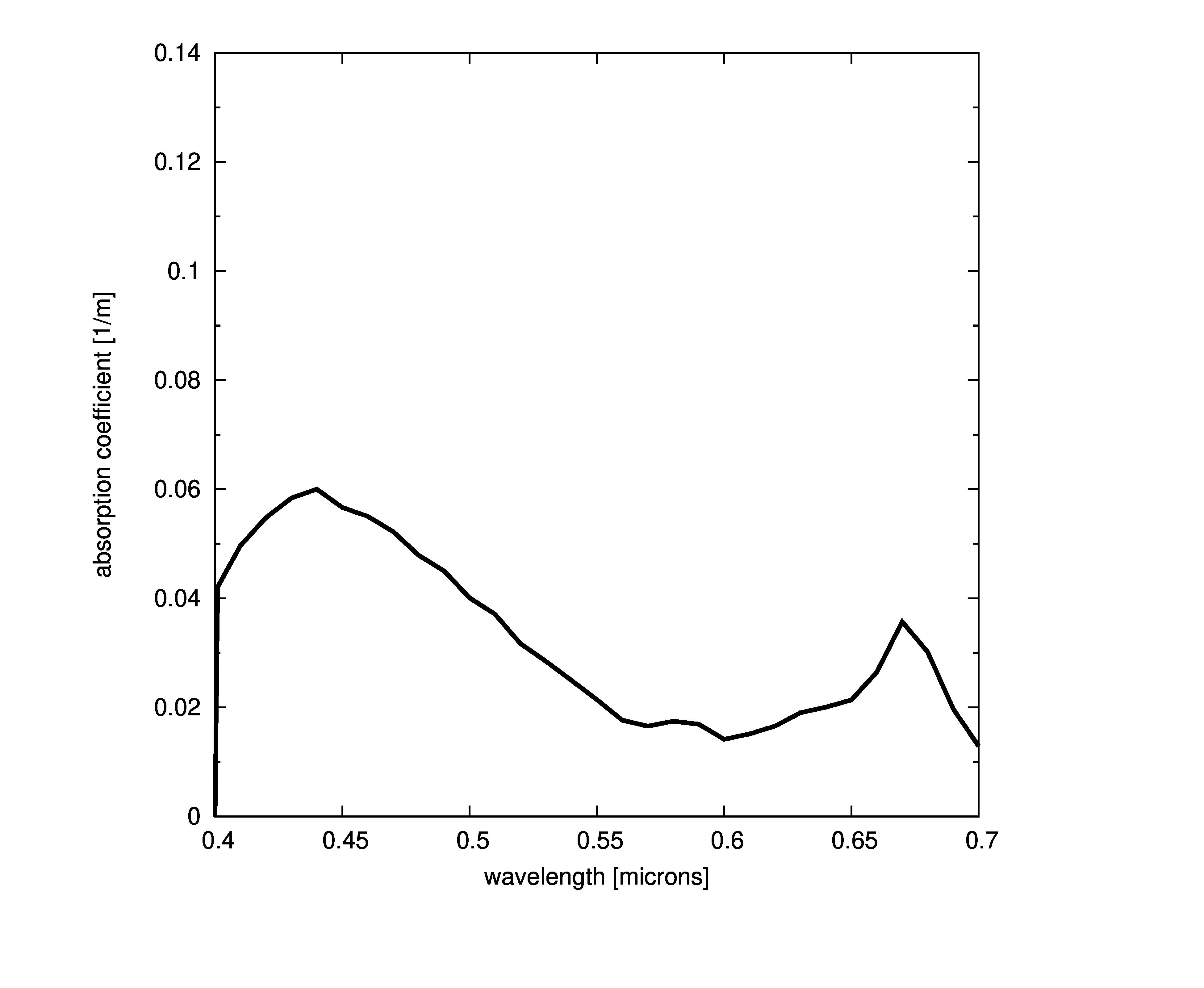
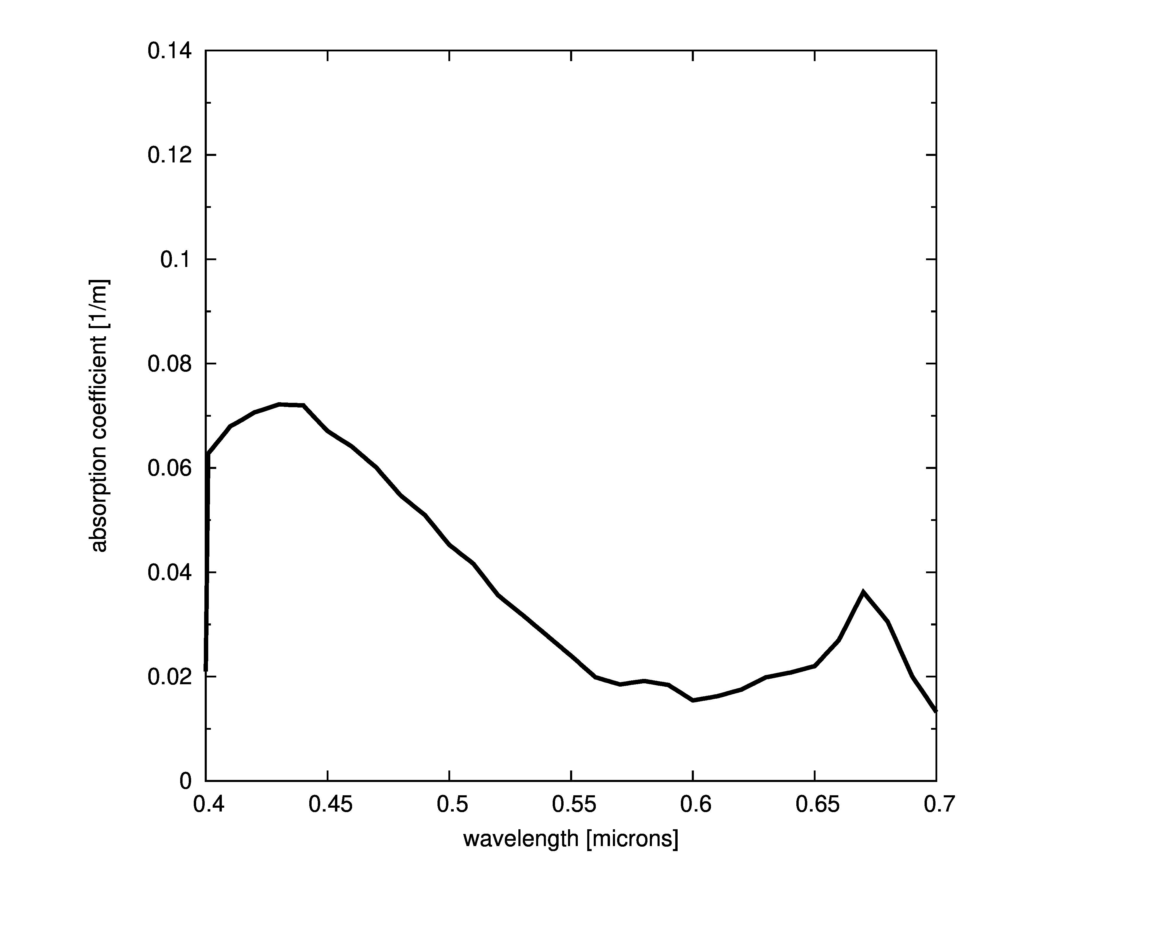
Plots of absorption coefficients using default values of all the models are given in the following plots. In cases where a concentration is part of the model, a constant value of 1.0 was used. Note that some of the models are only valid for the spectral range of [400-700] nanometers and are marked accordingly.

Figure 1. TYPE = constant

Figure 2. TYPE = specific

Figure 3. TYPE = morleconc

Figure 4. TYPE = morelocovar (w/ morelconc)

Figure 5. TYPE = raman

Figure 6. TYPE = sbpf

Figure 7. TYPE = smithbaker

Figure 8. TYPE = prieursathy

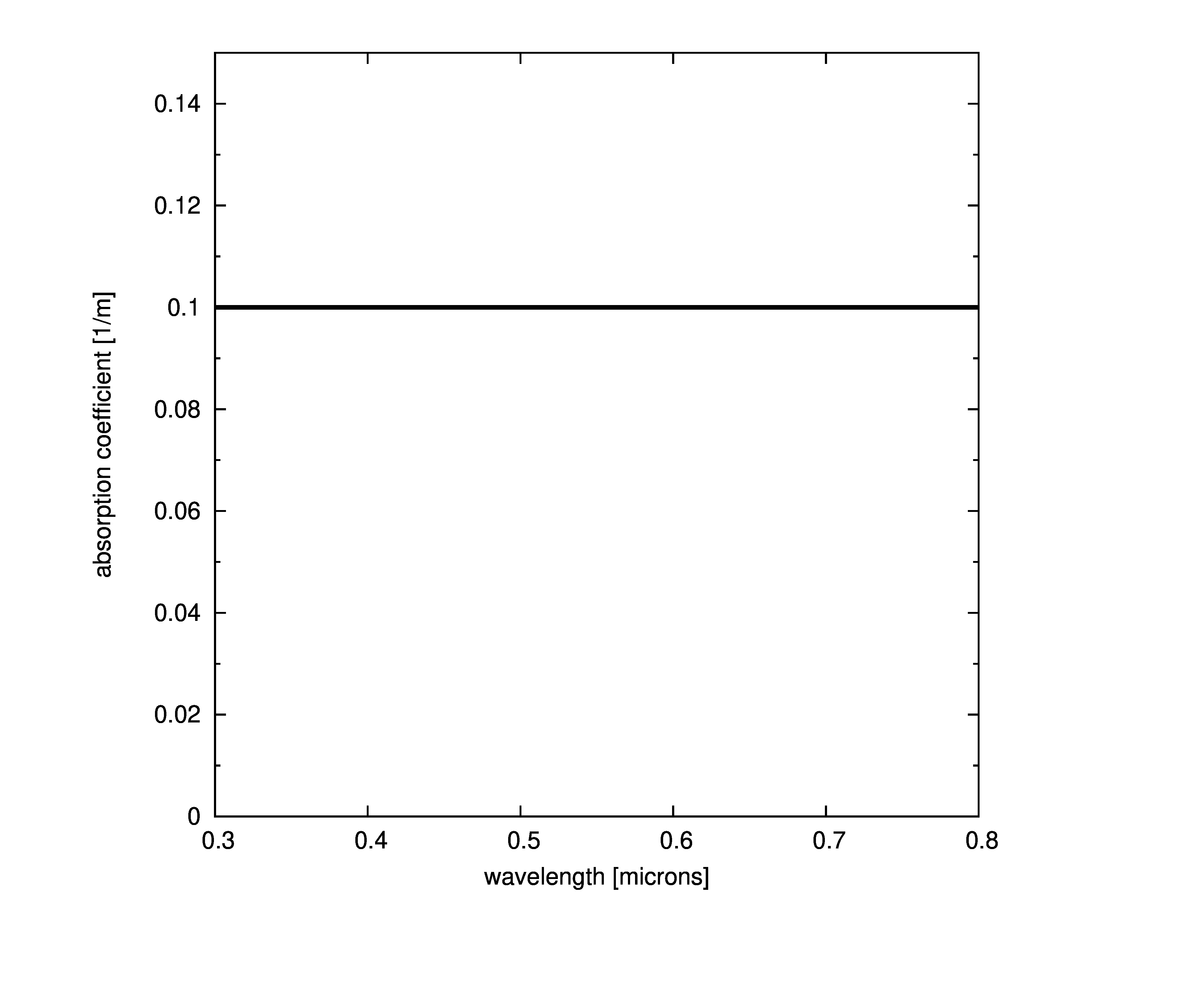
Constant absorption coefficient

The simplest way to define the absorption is to provide a file with the spectral absorption coefficients or provide a single coefficient that is constant across all wavelengths. This model assumes that the absorption coefficient is the same at any point in the medium ,

\[\begin{aligned} a(z,\lambda)&=&a(\lambda),\\\mbox{or}\\ a(z,\lambda)&=&a\label{eq: constantabs}. \end{aligned}\]

Specific absorption

In most cases, the primary IOP variation within a volume will be based on the local concentration of particulate matter. We will discuss how the spatial distribution can be described later in this manual. In the meantime, we need to establish the concept of a specific absorption coefficient, that is, an absorption coefficient that is independent of the concentration of particles. The relationship between the absorption coefficient, the specific absorption coefficient, and the concentration is expressed as

\[\begin{aligned} a(\vec{x},t,\lambda)&=&a^*(\lambda)C(\vec{x},t), \end{aligned}\]

where the superscript '*' is used to denote the "specific" nature of the parameter. Since the units of a are [1/m], care must be taken that the units of the concentration and the specific absorption coefficient result in the equivalent form. In practice, we will assume that we do not need to explicitly keep track of the time parameter and, similarly, the horizontal position only represents a different depth model. Thus, we will use the form

\[\begin{aligned} a(z,\lambda)&=&a^*(\lambda)C(z). \end{aligned}\]

For some of the models it will be necessary to normalize the specific absorption coefficient and obtain a non-dimensional representation. We will denote a normalized specific absorption coefficient by a'.

Specific absorption model

This absorption model is simply based on user-supplied specific absorption coefficients and the aforementioned optional noise parameter,

\[\begin{aligned} a(z,\lambda)&=&a^*(\lambda)C(z)\label{eq: specificabs}. \end{aligned}\]

Once again, care must be taken so that the units of the absorption coefficients and the concentration units are appropriate (no internal units checking is performed).

Morel based models

Two absorption models are based on the form given by ,

\[\begin{aligned} a(z,\lambda)&=&\left[a_w(\lambda)+0.06a_c^{*'}(\lambda)C_{chl}(z)^{0.65}\right]\left[1+0.2e^{-0.014(\lambda-440)}\right], \label{eq: morel} \end{aligned}\]

where a_w is the pure water absorption given above, \$a_c^{\mbox{*}}\$ is a non-dimensional chlorophyll-specific absorption coefficient derived by and normalized so that the value at 440 is equal to one, and \$C_{\mbox{chl}}(z)\$ is the chlorophyll concentration at depth z measured in \$[\frac{mg}{m^3}]\$. The wavelength, \$\lambda\$, is measured in nanometers ([nm]).

We shall follow Mobley’s lead and use a simplified reformulation of the Morel equation,

\[\begin{aligned} a(z,\lambda)&=&a_w(\lambda) + a_p(z,\lambda) + a_y(z,\lambda),\\ a_p(z,\lambda)&=&0.06a_c^{*'}(\lambda)C_{chl}(z)^{0.65},\\ a_y(z,\lambda)&=&0.2a_p(z,440)e^{-0.014(\lambda-440)}, \end{aligned}\]

where subscript p denotes chlorophyll particle absorption. It is apparent from the last two equations that there are two different types of models present; one model is concentration and specific absorption dependent, the other is covariant with another absorption coefficient.

Morel concentration

The Morel concentration model is given as

\[\begin{aligned} a(z,\lambda)&=&ka^{*'}(\lambda)C(z)^q. \end{aligned}\]

By default, the specific absorption coefficients do not need to be pre-normalized since the model will do so given the normalizing wavelength. Pre-normalized data can be used by turning the normalization off (the prenorm parameter, below).

Morel covariant

The third component of the Morel model leads to an expression for an absorption coefficient that covaries with another absorption coefficient. We can generalize the model as

\[\begin{aligned} a(z,\lambda)&=&ka_0(z,\lambda_0)e^{-q(\lambda-\lambda_0)}\label{eq: mcovariant}, \end{aligned}\]

where \$a_0\$ is the base absorption coefficient at \$\lambda_0\$, the base wavelength.

Raman "absorption" model

Though technically an (inelastic) scattering phenomenon, Raman scattering involves absorbing photons at a one wavelength and re-emitting them at another (longer) wavelength. Therefore, we will first handle Raman scattering as a loss from the beam via absorption. We will also allow the absorbed energy to reappear later on via a scattering method. Since the in-scattered contribution can only come from different wavelengths (instead of the wavelength of the current calculation), it makes sense to make this distinction. Mobley points out that there is a great deal of inconsistency in the literature regarding the exact formulation of Raman scattering, however, he presents the general form

\[\begin{aligned} a(\lambda)&=&a_0\left(\frac{\lambda_0}{\lambda}\right)^q\label{eq: raman}, \end{aligned}\]

where the 0 subscript refers to reference values (again see Mobley for a summary of current literature for this). We will use a recent set of measurements by for default values.

Raman scattering is a "quick" (instantaneous) inelastic process that is the product of immediate re-emission of light from water molecules.

Hybrid pure water data

This absorption model combines pure water data from both the finer resolution, but limited range, data from Pope and Fry, with the broader ranged, but coarser resolution data from Smith and Baker. The user interface to this model is simple since it just implements the data (with interpolation).

Smith-Baker pure water data

This model implements the pure water absorption data from directly. The user interface to this model is simple since it just implements the data (with interpolation).

Prieur-Sathyendranath pure water data

This model implements the pure water absorption data from directly, which can be used as an alternative data set. The user interface to this model is simple since it just implements the data (with interpolation).

Scattering coefficient models

Development of the scattering coefficient models is analogous to absorption coefficient models. We define two essential, basic models ("constant" and "specific", as above) as well as two based on the basic forms of established concentration relationships. Scattering coefficient models are added to a base medium which may or may not define initial scattering properties. All scattering coeffcient models are combined linearly to produce the final coefficient at any point. To add a scattering model, the user adds an ADD_SCATTTERING_MODEL sub-section to the IOP model section of the material file. The first entry within this subsection is:

TYPE = <model type>

ADD_SCATTERING_MODEL {
    TYPE = gordonmorel
    ID = chlScat
    K = 0.33
    Q = 0.62
    CONCID = chlConc
    EXCLUSIVE = 0
 }

Plots of scattering coefficients using default values of all the models are given in Figure #fig: scatmodelplots[[fig: scatmodelplots]]. In cases where a concentration is part of the model, a constant value of 1.0 was used.

As with the absorption coefficient models, each scattering model independently implements the general CDScatteringProperty interface, but are used indirectly through the linear scattering model (PMLinearScatModel). Figure #fig: scatclassmap[[fig: scatclassmap]] shows the relationship between the models and DIRSIG interfaces.

Constant scattering coefficient

This model assumes that the scattering coefficient is the same at any point in the medium (though the noise parameter may add some variation) and potentially constant across wavelengths,

\[\begin{aligned} b(z,\lambda)&=&b(\lambda),\\ \mbox{or}\notag\\ b(z,\lambda)&=&b\label{eq: constantscat}. \end{aligned}\]

Specific scattering model

This scattering model is simply based on user-supplied specific scattering coefficients (see the section on specific absorption, above) and the optional noise parameter,

\[\begin{aligned} b(z,\lambda)&=&b^*(\lambda)C(z)\label{eq: specificscat}. \end{aligned}\]

Once again, care must be taken so that the units of the scattering coefficients and the concentration units are appropriate (no internal units checking is performed).

Gordon-Morel based model

We will follow the approach taken for the absorption models and attempt to derive generic model types based on established models. In this case, we look at the model for scattering from and (the latter work added the pure water term),

\[\begin{aligned} b(z,\lambda)&=&b_w(\lambda)+\left(\frac{550}{\lambda}\right)0.30C_c(z)^{0.62}, \end{aligned}\]

where the wavelength, \$\lambda\$, is in nanometers and \$C_c\$ is the chlorophyll concentration in [\$mg m^{-3}\$]. This simple formulation suggests a model of the form

\[\begin{aligned} b(z,\lambda)&=&\left(\frac{\lambda_0}{\lambda}\right)k\cdot C(z)^q\label{eq: gmconcentration}. \end{aligned}\]

Kopelevich based model

A scattering coefficient model by is given by

\[\begin{aligned} b(z,\lambda)&=&0.0017\left(\frac{550}{\lambda}\right)^{4.3}+ 1.34\nu_s(z)\left(\frac{550}{\lambda}\right)^{1.7}+ 0.312\nu_\ell(z)\left(\frac{550}{\lambda}\right)^{0.3}, \end{aligned}\]

where \$\nu_s\$ and \$\nu_\ell\$ are the concentration of small and large particles in ppm. Even though this model for the scattering coefficient folds in the pure water scattering, we accept it as a general model form. Consequently, our model is

\[\begin{aligned} b(z,\lambda)&=&k\cdot C(z)\left(\frac{\lambda_0}{\lambda}\right)^q\label{eq: kconcentration}, \end{aligned}\]

where we will make the concentration an optional parameter.

Buiteveld model

The pure water scattering model based on was already presented in Section #sec: basemedium[1.3]. This model is directly available to the user via the buiteveld scattering model.

Raman scattering

Implementation of Raman scattering and, more specifically, the wavelength distribution models would involve a complex mixture of photon mapping estimation, IOP definition, and LUT integration. We will put aside the development of this model for future development.

Scattering phase function models

The scattering phase function is essentially a PDF in spherical coordinates that describes where scattered photons go. We will make the common assumption that all scattering phase functions are rotationally symmetric around the forward direction (direction of propagation). This enables us to sample the phase function shape (the angle, \$\theta\$) using the simple, one-dimensional importance sampler or an analytical model coupled with uniformly sampling the rotation angle (\$\phi\$). We will also assume that there is no spectral dependence (the inherent spectral dependence of scattering is expressed by the scattering coefficient).

When providing phase function data, it is useful for the user to get in the habit of sampling on constant cosine intervals, \$\mu\$, where the angle, \$\theta=\cos^{-1}(\mu)\$. This method of sampling facilitates numerical integration and sampling in spherical coordinates since

\[\begin{aligned} \int_0^{2\pi}\int_{-1}^1 f(\mu,\phi)d\mu d\phi&=&\int_0^{2\pi}\int_{\pi}^{0}f'(\theta,\phi)dcos(\theta)d\phi\notag\\ &=&\int_0^{2\pi}\int_0^\pi f'(\theta,\phi) sin(\theta)d\theta d\phi, \end{aligned}\]

which gives us the correct form of the integral in spherical coordinates without having to weight the \$\theta\$ intervals. While this form is preferred, the phase function routines will convert \$\theta\$ samples to \$\mu\$ samples if necessary (based on a type flag in the input).

All of the scattering phase functions must have an associated scattering coefficient model. In cases where no SPF is provided for a coefficient model, a uniform SPF is used. Scattering phase function models are added to a base medium which may or may not define initial scattering properties. All scattering phase function models are combined linearly (weighted by the corresponding scattering coefficients) to produce the final SPF at any point. To add a scattering phase function model, the user adds an ADD_PHASE_FUNCTION_MODEL sub-section to the IOP model section of the material file. The first entry within this subsection is:

TYPE = <model type>

where <model type is the unique type name for the IOP model (given within the tables). This is different from the ID parameter that is used to differentiate between models of the same type. Parameter entries follow, as seen in this example (for the Petzold average particle (petzold) model).

ADD_PHASE_FUNCTION_MODEL {
    TYPE    = petzold
    SCATID  = chlScat
}

The Petzold phase function is shown below.

Uniform model

The first scattering phase function model simply associates an equal weighting to all directions, i.e.

\[\begin{aligned} \tilde{\beta}(\mu,\phi)&=&\frac{1}{4\pi},\label{eq: uniformbeta}\\ \int_0^{2\pi}\int_{-1}^{1}\frac{1}{4\pi}d\mu d\phi &=& 1. \end{aligned}\]

User-Supplied data model

This model allows the user to provide phase function data on \$\theta\$ or \$\mu\$ samples. The user should ensure that the phase function is appropriate, that is, the integral of the function over \$\theta\$/\$\mu\$ (i.e. the angle from the forward direction) is \$\frac{1}{2\pi}\$, so that the total integral is one (rotational symmetry is assumed).

Henyey-Greenstein phase function model

The Henyey-Greenstein phase function is a very useful function to use since it is simple to analytically invert for sampling. However, phase functions of natural waters can only be described by using many of these functions in weighted combination. This model allows the user to define the component function (characterized by the average cosine, g) and the corresponding weights, i.e.,

\[\begin{aligned} \tilde{\beta}(\theta,\phi)&=&\sum_{i} w_i\tilde{\beta}_{hg,i}(\theta,\phi,g_i). \end{aligned}\]

The weights will be normalized internally so there is no need to ensure that they sum to one.

Schlick phase function model

The Schlick phase function is similar to the Henyey-Greenstein model, but it is slightly more efficient to calculate. The defining parameter, k, is analogous to g, but is not exactly equivalent to the average cosine. Once again, we implement the model as a linear combination of functions.

Rayleigh based model

We already saw a Rayleigh-like phase function in the description of pure water. We now add a generic form of this equation to our models,

\[\begin{aligned} \tilde{\beta}(\theta,\phi)&=&k_1(1+k_2\cos^2(\theta))\label{eq: rayleighlike}. \end{aligned}\]

Note that the user is responsible for choosing \$k_1\$ and \$k_2\$ so that the function is normalized.

Petzold scattering phase function data

The commonly used Petzold average particle scattering phase function data is implemented as the petzold phase function model.

Refractive index models

The refractive index model is the first of two IOP models that do not add linearly internally. In this case, there is only allowed to be one refractive index model at a time and each model provides the implementation of the general refractive index property. To define a new refractive index model to be used (overriding the refractive index in the based medium), the user adds a REFRACTIVE_INDEX_MODEL sub-section to the IOP model section of the material file. The first entry within this subsection is:

TYPE = <model type\'>

where <model type is the unique type name for the IOP model (given within the tables). As with the other IOPs, parameter entries follow, as seen in this example (for the constant refractive index (constant) model).

REFRACTIVE_INDEX_MODEL {
    TYPE = constant
    IOR = 1.34
}

Constant refractive index model

The constant refractive index model allows the user to define an index of refraction that is constant across all wavelengths (such as the one used in Hydrolight).

The IAPWS refractive index model

The IAPWS refractive index model was already mentioned previously as part of the base medium. Though the details will not be presented here, it implements the model described in the manual. The implementation is a two parameter model where the user is able to define the temperature and density of the medium.

Aggregate concentration models

Many of the IOP models presented previously make use of the local concentration of a particular constituent to determine their value at a point in space. In fact, this is currently the only way to vary IOP properties spatially, though there is nothing in the code that restricts a directly spatially variant model in the future (though this would be difficult to define). Though multiple concentration models can be implemented in the same space, they do not combine linearly as with most of the other IOPs. Instead, the concentration models exist independently in aggregate so that the concentrations of multiple constituents (e.g. chlorophyll, suspended sediments, etc…) can be defined independently from each other. For example, the following material file snippet defines three independent constituent concentration models:

IOP_MODEL {
...
    ADD_CONCENTRATION_MODEL {
          TYPE = gauss
          ID = chlConc
          BG = 0.2
          S = 9
          H = 144
          DMAX = 17
          ZLEVEL = 0
    }
    ADD_CONCENTRATION_MODEL {
        TYPE = constant
        ID = ssConc
        CONC = 0.1
    }
    ADD_CONCENTRATION_MODEL {
        TYPE = constant
        ID = cdomConc
        CONC = 0.5
    }
...
}

Currently, the definition of the distribution of concentrations is restricted to vertical variability only in order to simplify the input format. This was done because it is not yet clear what type of three-dimensional data will be available for future studies (as might be provided by a hydrodynamics model). Rather than attempt to guess at a useful data format, implementation of a fully three-dimensional concetration field will remain future work.

Constant concentration model

The constant concentration model acts as expected, providing an unchanging value througout te

Gaussian concentration model

The Gaussian concentration model corresponds to a concentration depth profile presented in that is used to model the concentration of chlorophyll measured in the Celtic Sea in May. The depth profile has the form:

\[\begin{aligned} C(z)&=&C_o + \frac{h}{s\sqrt{2\pi}}\exp{\left[-\frac{1}{2}\left(\frac{z-z_{\mbox{max}}}{s}\right)^2\right]},\label{eq: gaussianconc} \end{aligned}\]

which we will use as the general description of a Gaussian profile. The peak of the concentration curve is present at a depth of \$z_{\mbox{max}}\$ (DMAX in the user interface) and there is always a minimum background concentration of C_o (BG). The default parameters given for the model match those used to fit the Celtic Sea data.