This document provides a brief outline of the basic design of the DIRSIG radiometry model and supporting modules.
Model Overview
The Digital Imaging and Remote Sensing Image Generation(DIRSIG) model has been actively developed at the Digital Imaging and Remote Sensing (DIRS) Laboratory at Rochester Institute of Technology (RIT) for two decades. The model is designed to generate passive broadband, multi-spectral [1], hyper-spectral [2] low-light [3], polarized [4], active laser radar [5], and synthetic aperture radar [6] datasets through the integration of a suite of first-principles based radiation propagation modules. These object oriented modules address tasks ranging from bi-directional reflectance distribution function (BRDF) predictions of a surface, to time and material dependent surface temperature predictions, to the dynamic viewing geometry of scanning imaging instruments on agile ground, airborne and space-based platforms. In addition to the myriad of DIRSIG specific modules that have been created, there is a suite of interface modules that leverage externally developed atmospheric (e.g. MODTRAN) and thermodynamic (e.g. MuSES) components that are modeling workhorses for the multi-and hyper-spectral community. The software is employed internally at RIT and externally within the user community as a tool to aid in the evaluation of sensor designs and to produce imagery for algorithm testing purposes. Key components of the model and some aspects of the model’s overall performance have been gauged by several validation efforts over the past decades of the model’s evolution. [7]
The DIRSIG radiometry engine is very robust and modular. To produce data sets that contain the spatial and spectral complexity of real-world data, the model must be able reproduce a large set of radiative mechanisms that combine to produce the spectral signatures that are collected by real-world imaging instruments. The DIRSIG model attempts to incorporate a wide array of these image-forming processes within one modeling environment. To drive these predictive codes, the model must have access to robust characterizations of the elements to be modeled. For example, input databases describe everything from the chemical description of the atmosphere as a function of altitude to the spectral covariance of a specific material in the scene.
The current DIRSIG software is written entirely in C++ (a C++17 compliant compiler is required) and is managed with revision control system and continuous integration. The model includes a detailed graphical user database and is available for a wide variety of computing platforms including Windows, MacOS and Linux. Updates to the software are released 3-5 times a year to a user base of users working for the U.S. Government either directly or at supporting contractors.
History
The DIRSIG model has been under development since the late 1980s. However, the software has undergone multiple, ground-up rewrites since it’s inception. The brief timeline outline below summarizes the history of code development.
- DIRSIG2
-
Internally started in 1998. Limited external distribution. Blend of C and Fortran (THERM temperature prediction code). Final release was 2.9.2 in 1996.
- DIRSIG3
-
First publically distributed version. Entirely C/C++ (Fortran → C conversion for THERM temperature prediction code). First released in 1997. Final release was 3.7.3 in 2003.
- DIRSIG4
-
Entirely C++ (legacy Fortran code was rewritten as C++). First released in 2002. Final development release was 4.7.5 in 2019. Maintenance updates are included in current releases.
- DIRSIG5
-
Current development efforts. Entriely C++17. First beta releases in 2017 and general release in 2020. This is the current, actively developed version of DIRSIG.
Since DIRSIG5 does not support some features that DIRISG4 did (and vice-versa) the following comparison can be useful.
Light Transport Algorithm Basics
Basic Ray Tracing
The DIRSIG radiometry engine is driven by a ray tracer which finds intersections with geometric elements within the scene. A ray is defined by a direction vector, an origin that it emanates from and (optionally) a length. The geometry of the scene can be described by planes (infinite extent), facets or polygons (planes with finite extent), and other mathematical primitives including spheres, boxes, cylinders, etc. An intersection calculation is simply finding the mathematical solution to where the ray equation and the equation for the geometric object intersect (for example, the point where the equation for a line and a plane intersect). In it’s most primitive form, a ray tracer works by identifying objects that intersect a given ray through a brute-force search. However, once the number of scene objects becomes large, this approach becomes computationally inefficient. The DIRSIG ray tracer employs a variety of spatial sorting optimizations that minimize the number of geometric objects that must be checked for intersection.
Forward and Reverse Ray Tracing
In most cases DIRSIG employs "reverse ray tracing", where rays are traced into the scene from the sensor looking at the scene. In this approach, the ray tracer quickly finds objects that can be seen by the sensor, but strategies must be employed to figure out the illumination onto those objects. DIRSIG also employs "forward ray tracing", where rays are traced into the scene from the "sources" (e.g. the sun, the moon, the sky, user-defined sources, etc.). In this approach, strategies must be employed to figure out which objects can be seen by the sensor. Finally, DIRSIG utilizes some hybrid approaches that employ both forward and reverse ray tracing.
|
|
Ray tracing is simply the process of following rays and figuring out what they intersect. Ray tracing itself is not a rendering method itself, but rather a tool used to compute terms in a rendering equation. |
Using Ray Tracing for Light Tranport Algorithms
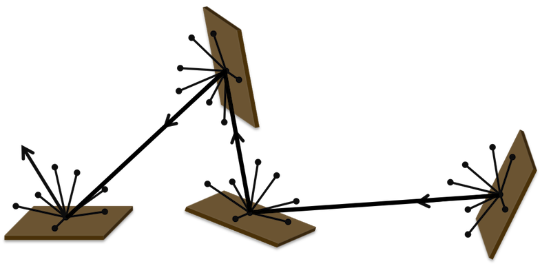
"Whitted-style" Ray Tracing
A limited number of rays are shot from the sensor (enough to spatially sample the directly viewable geometry within the pixel IFOV), but at each surface the view ray spawns multiple sampling rays to determine the incident flux onto that surface and how much is reflected into the viewed direction. Those sampling rays can find other surfaces, which are similarly sampled. This method is generally credited to Turner Whitted [8] and it sometimes referred to as "Whitted-style" ray tracing. The implementation of these surface calculations can insure that the sampling for later bounces is decreased to make the sampling not grow exponentially.
DIRSIG4 and previous generations of DIRSIG generally employed this approach to ray tracing to solve for the light transport within the scene.
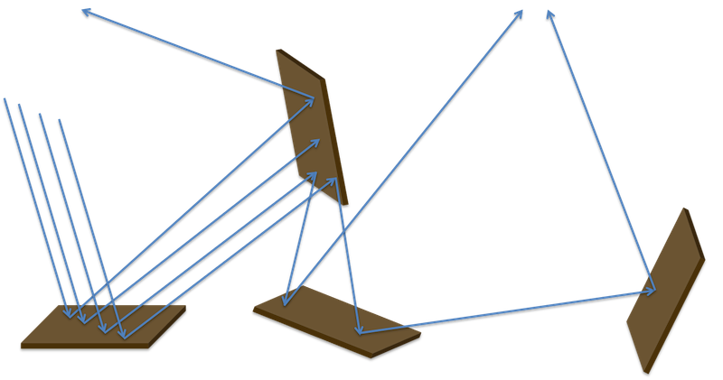
Path Tracing
Path tracing is a rendering approach where a ray starts at the detector and intersects an object in the scene. Monte-Carlo techniques are then employed to figure out if the ray is absorbed, reflected or transmitted. If it is absorbed, then the propagation ends. If the ray is either reflected or transmitted, then the reflectance or transmission model for the surface is used to figure out which direction the ray should continue in. A specular reflector has a higher probability of the ray continuing in a perfect "mirror" direction whereas a diffuse reflector favors the ray leaving in a random direction. Mechanisms can be employed to make sure that important sources in the scene are considered in the leaving ray direction. An initial ray that ultimately is absorbed returns nothing, but a ray that ultimately finds a source returns the flux from that source reflected through the chain of surfaces leading from the source to the sensor. A large number of rays must be shot from the sensor to build up a low-noise flux reaching the sensor. Each ray takes a different random walk through the scene geometry to the various sources (for example, the sun, the moon, the sky) illuminating the scene. This approach is generally considered to be an "infinite bounce" approach, although implementations can enforce limits on the number of bounces to track before assuming the ray never reaches a source.
DIRSIG5 employs a "path tracing" approach to solve for the light transport within the scene.
Whitted-style Ray Tracing vs. Path Tracing
The justification for the migration in DIRSIG5 to "path tracing" from the previous "Whitted-style" approaches is best summarized by this explanation:
Since Whitted-style ray tracing originates multiple rays at each ray-object intersection, computation is spent on deeper parts of the tree of rays. An important property of path tracing vice Whitted-style ray tracing is the computational emphasis on the low-depth (fewer bounce) rays. Since, generally, low-depth rays contribute more to the resulting image than high-depth rays, path tracing’s computation time is proportionate to the resulting contribution.
University of Texas at Austin Computer Science
DIRSIG5 Details
DIRSIG5 represents a rewrite of the over 500,000 lines of code in DIRSIG4 to produce a new DIRSIG model that features higher radiometric and computational performance. The following sections attempt to briefly describe the major differences between the two versions of the software.
Plugin-Based Architecture
The DIRSIG5 software is constructed and deployed differently than DIRSIG4 was. DIRSIG5 is constructed around a arelatively stable "radometry core" and most features are provided via a series of plugins rather than features to a monolithic compiled code. This helps provide feature modularity and allows the radiometry core to establish stable and well tested APIs through which these plugins communicate to the radiometry engine. The current DIRSIG5 software includes a set of plugins that provide backward compatibility with existing DIRSIG4 simulation configurations. The list of the documented plugins employed by DIRSIG5 can be found in the plugins manual.
Improved and Simplified Radiometry
In DIRSIG4, the speed and fidelity of the simulation could be controlled through a series of configuration choices and settings spread across the material configurations and sensor modeling parameters. The two primary mechanisms utilized by users were:
- Radiometry Solver Configurations
-
Radiometry solvers are the algorithms that performed the surface (or volume) leaving radiance calculations. The user could select a lower fidelity radiometry solver or dial down the parameters of a higher fidelity solver to decrease fidelity and improve run times.
- Sub-Pixel Sampling Configurations
-
Sub-pixel sampling defines how many sample rays were used in each pixel. The more rays that are used, the better the estimate of the diversity and proportion of radiance signatures that are present within the collection area of the pixel. However, using more sub-pixel rays linearly correlates with run-time.
In general, users were often observed dialing down the fidelity of a DIRSIG4 simulation (using these two mechanisms) in order to meet compute time targets. Furthermore, there wasn’t an easy "single knob" interface to DIRSIG4 to control the fidelity vs. time trade off.
In DIRSIG5 there are no radiometry solvers because it utilizes a new, unified numerical radiometry calculation. DIRSIG5 uses path tracing, which follows a single ray path from the pixel to either a source of energy (sun, moon, sky, light, etc.) or a termination (absorbed). Since this approach is emulating a Monte-Carlo integral of all the light paths reaching a pixel, the fidelity of the solution is proportional to how many samples (paths) are used. This "number of paths" parameter provides the sought after single knob interface controlling fidelity vs. time for the model. When a small number of paths are used, the resulting radiance estimate will be noisy. As more paths are used, the estimate improves. Controlling the number of paths per pixel is discussed in the DIRSIG5 Command-Line Guide.
Multi-threaded Execution
Unlike DIRSIG4, the DIRSIG5 code is multi-threaded. That means more compute resources can be utilized for micro-scale parallelization on a multi-core computer. Controlling how many threads are used by the model is discussed in the DIRSIG5 Command-Line Guide.
Multi-computer Execution
DIRSIG5 releases include a Message Passing Interface (MPI) enabled executable that will allow the software to distribute computations on clustered computing resources. Details about using the MPI-enabled version of DIRSIG is described in a supplementary manual.
GPU Acceleration
Future releases of DIRSIG5 may utilize NVIDIAs CUDA and OptiX frameworks for GPU-accelerated ray tracing, which currently accounts for approximately 60% of the execution time. Numerous prototypes have been created but none of them have yielded a viable solution. Hence, DIRSIG5 is not GPU accelerated at this time.
Supporting Components
Scene Description
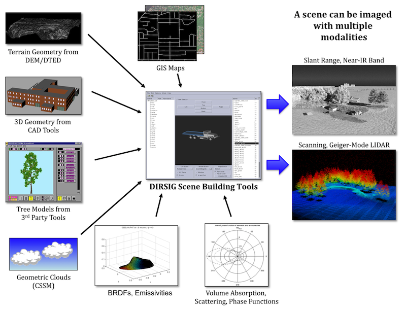
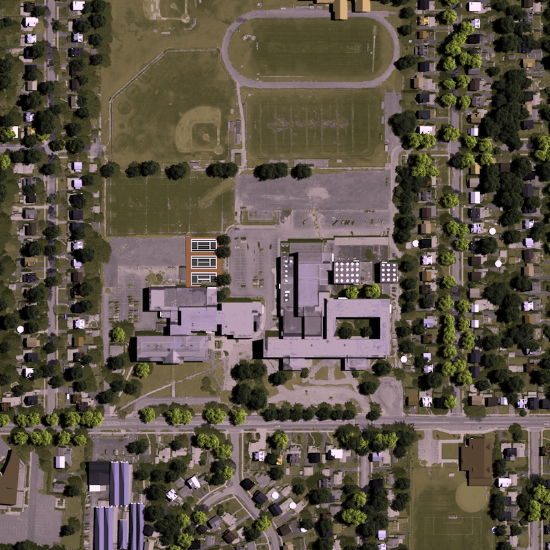
One of the key features of the DIRSIG model is that all modalities are simulated from a common scene description. The synthetic world that is employed is composed of 3-D geometric constructs (polygon geometry, mathematical objects and voxelized geometry) that are assigned a material description (see Figure 1). Users can create 3-D polygon models with a variety of 3-D asset creation tools including AutoCAD, 3ds Max, Rhinoceros, Blender3D, SketchUp, etc. This material description includes thermodynamic properties to enable temperature prediction and optical properties to drive the radiometric prediction. Instead of a discrete suite of modality specific models, the currently supported modalities all share the same geometric and radiometric core, which insures phenomenological agreement across modalities. For example, the same specular paint BRDF for a car hood would be used when simulating both a passive RGB camera and an active LIDAR system. If a vehicle is painted black, it will be warmer than a lighter colored material in the thermal infrared because of the differences in solar absorption. The scene database also supports dynamic object positioning, which allows objects like vehicles to be linked to external traffic simulators (for example, the Simulation of Urban MObility (SUMO) model) or collection scenario planning and management tools including System Toolkit (STK).
Instrument and Platform Modeling
The DIRSIG sensor module was designed to provide a framework upon which a myriad of multi-modal sensors could be implemented. Passive imaging systems can range in complexity from single-pixel scanning architectures, to modular pushbroom arrays to 2-D imaging arrays. The geometry (pixel sizes and locations) of an imaging array is separated from the "capture" of incident energy by that device. This allows a 2-D array to be combined with either an array wide filter or a color-filter array (for example, a Bayer pattern) to capture multi-spectral imagery. To model a hyper-spectral system, the same 2-D array can be combined with a dispersive or refractive element to create the spatial separation of the incident spectral flux. A LIDAR receiver array analyzes the incident temporal flux to determine when a return is detected. However, a real or synthetic aperture radar system employs an entirely different family of radiation measurement technologies. In these systems, the user is describing an antenna array and the radial gain function.
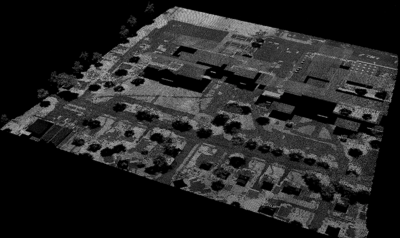
The DIRSIG model also features an advanced data acquisition model that centers on the concept of a "platform" that can have one of more imaging or non-imaging sensors attached to it. The platform model allows sensors to be positioned relative to one another and synchronized by central clocking mechanisms. This platform can represent a variety of data acquisition platforms ranging from a fixed tripod, to a driving van, to a flying aircraft to an orbiting satellite (Brown 2011). The platform model also supports flexible command data interfaces to control the position and orientation of the platform as a function of time (e.g. vehicle route, aircraft flight line, etc.) as well as dynamic platform relative pointing interfaces (scan patterns, camera ball pointing, etc.). The images in Figure 2 and Figure 3 are simulated data products for the same scene, but were collected by separate airborne LIDAR and color image systems. In addition to employing different sensor modalities, these two sensors were imaged from different platforms at different times of day.
The primary sensor and platform model in DIRSIG5 is provided by the BasicPlatform sensor plugin.
Technical Readiness Levels
The DIRSIG model can model a variety of different imaging modalities and application areas. These different focus areas have been independently developed over many years and with different levels of focus or resources. In order to help the end-user gauge the technical readiness of the model for a given application, we have developed a qualitative scale to rank different aspects of the model. These levels track the life cycle of a new modality or research application are from conception to maturity. The largest driver in how quickly something progresses through the lifecycle is community interest and resources. Some new model features are conceived and incubated during a period of intense interest by the community, which then wavers. In those cases, a topic might be abandoned until interest and funding resources are renewed.
Mature
This level represents the highest level of readiness on the scale. That does not mean that there is no room for improvement, but it does indicate that the application area has been well exercised by the team at RIT and the user community as a whole. Documentation and examples for this level are usually abundant.
Operational
This level corresponds to features that are becoming finalized. Documentation and demonstrations (examples) at this level are well established but (perhaps) not complete. End users should utilize features at this level with caution and expect minor bugs and well documented limitations.
Experimental
This level represents a capability that has achieved the most basic form of usability. Documentation for capabilities at this level are usually non-existent or ad-hoc. Interfaces to the model may change as the capability is refined and matured. End users should utilize features at this level with extreme caution and expect bugs and undocumented limitations.
Exploratory
This level is associated with new research areas that are being researched by the team at RIT, but which is not currently available to the end-user in any form. Some research in this area may never make it out of this state.
Current Status and Limitations
To date, the DIRSIG5 software effort has focused on radiometric and computational performance for EO/IR simulations. The following limitations exist at this time.
-
No Synthetic Aperture Radar (SAR) Capabilities
-
We have a white paper outlining the effort to get this active sensing modality supported under the new DIRSIG computational architecture.
-
To model this modality, the user can continue to use DIRSIG4.
-
-
No Polarization Capabilities
-
We currently has no plans to support this modality. The capability in DIRSIG4 was used by a very small fraction of the user population.
-
To model this modality, the user can continue to use DIRSIG4.
-