A key component of the DIRSIG model’s geometry support is the positioning and orienting various objects in 3D space. This concept includes the positioning of scene objects (see the ODB and GLIST files) as well as the platform (see the PPD file). The primary mechanism employed to perform this task is the affine transform, which is a combination of rotations, translations, scales (dilations) and shears. An affine transform has two very specific properties:
-
Collinearity is preserved
-
All points lying on a line still lie on a line after the transformation is applied.
-
-
Ratios of distances are preserved
-
The midpoint of a line segment remains the midpoint after the transformation is applied.
-
|
|
Historically the DIRSIG model hasn’t employed shear operations, although they are completely supported via any interfaces that allow the user to input the raw 4x4 affine transform. |
Common Transforms
The following section outlines the mathematics defining common operations applied to objects in the DIRSIG model. These operations will be defined in terms of how they operate on a 3D point, however the concept can be applied to entire 3D lines (defined by 2 or more points), 3D polygons (defined by 3 or more non-collinear points) or a 3D object (defined by 1 or more 3D polygons). However, most of this document will discuss a given transform M in terms of an operation on a point p, yielding the new point p':
\(p' = M p\)
Since the DIRSIG model addresses a 3D world, the operations will be defined in terms of the Euclidean X, Y and Z axes.
Translation
A translation operation will translate a point from an initial position to a new position based on a linear shift. For example, a point that is distance N from the origin can be translated a distance M such that the final distance is N+M.
The following equations define the 4x4 matrix for translation in the various axes.
\( M(t_x) = \left [ \begin{array}{cccc} 1 & 0 & 0 & t_x \\ 0 & 1 & 0 & 0 \\ 0 & 0 & 1 & 0 \\ 0 & 0 & 0 & 1 \\ \end{array} \right ] \)
\( M(t_y) = \left [ \begin{array}{cccc} 1 & 0 & 0 & 0 \\ 0 & 1 & 0 & t_y \\ 0 & 0 & 1 & 0 \\ 0 & 0 & 0 & 1 \\ \end{array} \right ] \)
\( M(t_z) = \left [ \begin{array}{cccc} 1 & 0 & 0 & 0 \\ 0 & 1 & 0 & 0 \\ 0 & 0 & 1 & t_z \\ 0 & 0 & 0 & 1 \\ \end{array} \right ] \)
A series of axis translation operations are commutative, hence the total translation for each axis in the series can be summed (translations are additive) and a single transform matrix capturing translations for all axes can be computed directly:
\( M \left ( \sum t_x, \sum t_y, \sum t_z \right ) = \left [ \begin{array}{cccc} 1 & 0 & 0 & \sum t_x \\ 0 & 1 & 0 & \sum t_y \\ 0 & 0 & 1 & \sum t_z \\ 0 & 0 & 0 & 1 \\ \end{array} \right ] \)
Scale
A scale operation will shift a point from an initial position to a new position based on a scaling. For example, a point that is currently a distance N from the origin can be scaled by 2 to increase that distance to 2N.
The following equations define the 4x4 matrix for scaling in the various axes.
\( M(s_x) = \left [ \begin{array}{cccc} s_x & 0 & 0 & 0 \\ 0 & 1 & 0 & 0 \\ 0 & 0 & 1 & 0 \\ 0 & 0 & 0 & 1 \\ \end{array} \right ] \)
\( M(s_y) = \left [ \begin{array}{cccc} 1 & 0 & 0 & 0 \\ 0 & s_y & 0 & 0 \\ 0 & 0 & 1 & 0 \\ 0 & 0 & 0 & 1 \\ \end{array} \right ] \)
\( M(s_z) = \left [ \begin{array}{cccc} 1 & 0 & 0 & 0 \\ 0 & 1 & 0 & 0 \\ 0 & 0 & s_z & 0 \\ 0 & 0 & 0 & 1 \\ \end{array} \right ] \)
A series of axis scale operations are commutative, hence the total scaling for each axis in the series can be combined (scales are multiplicative) and a single transform matrix capturing scalings for all axes can be computed directly:
\( M \left ( \Pi s_x, \Pi s_y, \Pi s_z \right ) = \left [ \begin{array}{cccc} \Pi s_x & 0 & 0 & 0 \\ 0 & \Pi s_y & 0 & 0 \\ 0 & 0 & \Pi s_z & 0 \\ 0 & 0 & 0 & 1 \\ \end{array} \right ] \)
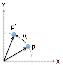
Rotation
A rotation operation will shift a point from an initial position to a new position based on a rotation about a given axis. For example a point that currently has an angle of theta between a line drawn from the point back to the origin and a reference axis can be rotated about an axis normal to the plane so that the new position forms a new angle to that reference axis.
The following equations define the 4x4 matrix for rotation in the various axes. Note that the signs of rotation angles are defined using a right-hand rule convention.
\( M(\theta_x) = \left [ \begin{array}{cccc} 1 & 0 & 0 & 0 \\ 0 & \cos( \theta_x ) & -\sin( \theta_x ) & 0 \\ 0 & \sin( \theta_x ) & \cos( \theta_x ) & 0 \\ 0 & 0 & 0 & 1 \\ \end{array} \right ] \)
\( M(\theta_y) = \left [ \begin{array}{cccc} \cos( \theta_y ) & 0 & \sin( \theta_y ) & 0 \\ 0 & 1 & 0 & 0 \\ -\sin( \theta_y ) & 0 & \cos( \theta_y ) & 0 \\ 0 & 0 & 0 & 1 \\ \end{array} \right ] \)
\( M(\theta_z) = \left [ \begin{array}{cccc} \cos( \theta_z ) & -\sin( \theta_z ) & 0 & 0 \\ \sin( \theta_z ) & \cos( \theta_z ) & 0 & 0 \\ 0 & 0 & 1 & 0 \\ 0 & 0 & 0 & 1 \\ \end{array} \right ] \)
Unlike the translation and scaling operations, a series of axis rotations are not commutative. That means that rotating a point about the X axis and then the Y axis yields a different result than if you rotate about the Y axis and then the X axis.
\(M(\theta_y) M(\theta_x) \neq M(\theta_x) M(\theta_y)\)
|
|
The order "X, then Y" must be translated into a matrix math form, where the matrix multiplication operations are performed right to left. Hence, "X, then Y" results in an equation that looks like \(p' = M_y \cdot ( M_x \cdot p )\). |
Transform Sequences
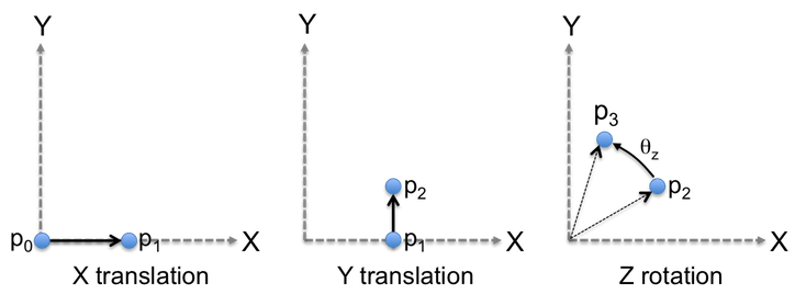
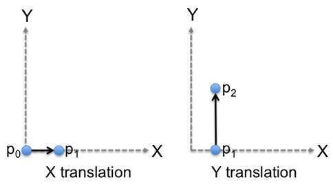
This section explains how an arbitrary sequence of translation, scale and/or rotation operations can be combined. The key concept is that the result of the previous operation is the input to the next operation. Consider the following sequence of operations that start with a point at the origin:
-
The point p0 is translated from the origin in the X dimension to the point p1.
-
The point p1 is translated in the Y dimension to the point p2.
-
The point p2 is rotated about the Z axis to the point p3.
This sequence of operations can be combined into a single affine transform matrix by combining the transform matrices in the correct mathematical order:
\(M = M(\theta_z) ( M(t_y) ( M(t_x) ) )\)
Sequence Equality
By looking at the final state of the operation sequence (p3) described in the previous section, the reader can see that the p0 to p3 transform could be accomplished by a simpler set of operations:
-
The point p0 is translated from the origin in the X dimension to the point p1.
-
The point p1 is translated in the Y dimension to the point p2.
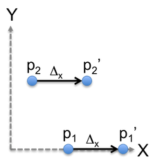
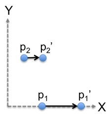
Although this results in the final point being in the same location, the sequences are only equivalent when applied to a single point. Consider the same pair of sequences again for square object, where the transforms modify the points defining the corners of the square:
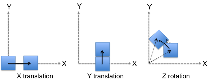
Now consider the simplified transform consisting of only X and Y translations:
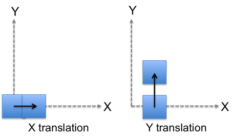
Notice how the final location of the square is the same between the two sequences but orientation is not. This is an important property to consider when affine transforms are utilized with collections of points like those in lines, polygons and collections of polygons.
|
|
In general, a complex set of operations results in a final state that is unique to that set of operations and the order that they were applied in. |
Interpolation
It is very common to want to interpolate between a set of states described by affine transforms. For example, a car driving down a road might be described by a series of states at different waypoints. Each state would include the location (a set of translation operations) and an orientation (a set of rotation operations). To determine the location and orientation of the car between the waypoints, the location and orientation must be interpolated from the neighboring known states. Although an 4x4 affine transform composed of just translation and/or scale operations can be linearly interpolated by weighting the elements in the 4x4 matrix, a transform containing rotations cannot. Instead the axis translations, scales and rotations must be interpolated and the affine transform matrix generated from the resulting values. It is important to note that this approach is only valid if the order of the rotation operations between the two know waypoints are the same.
|
|
One of the advantages to using quaternions is that there is a scheme for interpolating an arbitrary sequence of rotations directly. Support for quaternions will be added in future versions of DIRSIG. |
Affine Transforms in Use
This section briefly discusses how affine transforms are used in different parts of DIRSIG.
Object Instances
Platform Attachments
A mount attachment (to the respective platform) and an instrument attachment (to the respective mount) is an affine transform. This is an arbitrary sequence of translation and rotation operations, although scale operations are not usually employed (they do not make sense in the physical metaphor of the platform).
Platform Orientation
The PPD file describes the platform orientation as a sequence of X, Y and Z rotations. The user can specify the order of the rotations, but there is a single rotation for each axis.