The ChipMaker Plugin

Summary

This plugin was created to streamline the generation of image chips with "labels" to be fed into machine learning (ML) algorithms. In order to facilitate robust training, we want to generate a large number of image chips across a wide range of acquisition parameters. Those include:

Different targets and/or variants of targets
Different backgrounds (the context within which the target appears)
Different ground sampling distances (GSDs)
Different sensor view angles (zenith and azimuth)
Different illumination angles (zenith and azimuth)

Historically this has been accomplished using external scripting with a conventional DIRSIG simulation. The primary goal of this plugin is to make it easy to configure all the degrees of freedom in one location and have the plugin manage the creation of the images.

This plugin makes several assumptions and employs simplifications in how it models some elements of the simulation. Most of these choices were made in light of what training data and test data for ML algorithms looks like. Specifically that most ML workflows employ 8-bit and/or 24-bit images and various physical parameters of the sensor, scene, atmosphere, etc. are generally irrelevant. For example, the algorithm isn’t aware of the size pixels on the focal plane and the effective focal length. But it is aware of the GSD of the images. Likewise, the algorithm isn’t explicitly aware of a hazy maritime atmosphere vs. clear desert atmosphere. But it is aware that some images have lower contrast and some images have higher contrast. In light of the context of how these images are generally used in ML workflows, many of the approaches employed in this plugin have been simplified to streamline the setup of these simulations.

Camera Modeling

The modeling of the camera has been simplified to avoid the user needing detailed system specifications that are largely irrelevant in the context in which the output images are used. For example, the user defines the GSD directly rather than the physical size of pixel elements on the focal plane and an effective focal length. As a result, the object to image plane projection is orthogonal rather than perspective. Because the final imagery (the PNG, JPEG, etc. images used with the ML algorithm) won’t have physical units, it is not important to have detailed spectral response functions for each channel. Hence, the definition of spectral channels is limited to a simple bandpass defined by an lower and upper wavelength and the response is assumed to be uniform across that bandpass. There are options to incorporate the effective point-spread function (PSF) of the system, but that PSF is currently assumed to be constant across all channels.

Atmospheric Modeling

The ChipMaker plugin in DIRSIG5 is technically a combo plugin because it binds to both the sensor API (to drive the image formation) and the atmosphere API (to drive the source direction, direct illumination and diffuse illumination). This plugin offers two approaches to atmospheric modeling, depending on the required fidelity. Neither is a fully physics-driven approach:

The default model is a simple analytical model. The total irradiance from the hemisphere is spectrally constant and partitioned between direct and diffuse components. There is no path scattering or path transmission between the sensor and the scene. For a physics-based, remote sensing simulation tool this seems like an inappropriate simplification of the real world. However, utilizing a physics-based atmosphere model (for example, MODTRAN) would entail an enormous amount of computations since every chip would involve a unique view and illumination geometry. At this time, the reality is that calibrated images are rarely used to either train ML algorithms and ML algorithms are rarely supplied calibrated image to analyze. Hence, it doesn’t matter if the exact transmission and scattering is modeled because the algorithms are typically working with 8-bit, 24-bit, etc. images where the impacts of path transmission and scattering manifest as relative contrast differences in the image. Therefore, the approach here is to capture the multiplicative transmission loss and additive scattering gain in the conversion from output reflectance to integer count images. For example, a hazy atmosphere (high scattering, low transmission) can be emulated as a linear radiance to counts scaling that has a lower gain and higher bias when compared to a clearer atmosphere.
If more fidelity is required, a higher fidelity approach to atmospheric modeling is offered, called the FourCurveAtmosphere. This approach is an approximation of atmospheric effects through four spectral curves that are a function of solar zenith angle. The four curves are: (1) the ground-reaching solar irradiance, (2) the path radiance per unit distance, (3) the path extinction per unit distance and (4) the hemispherically integrated sky irradiance. This approach improves upon the simple parametric model while not requiring massive atmospheric radiative transfer computations unique for each chip. This plugin utilizes a pre-computed atmospheric database and each DIRSIG release includes a ready-to-run database containing a large number of atmospheric conditions. Alternatively, the user can generate their own database of conditions using the fourcurve_builder tool.

Input

The input file for the plugin is a JSON formatted file. An example file is shown below and will be discussed section by section. See the ChipMaker2 demo for a working example.

Example of a JSON document for the ChipMaker plugin.

{
  "atmosphere" : {
    "database" : "./my_atm_db.hdf",
    "conditions" : [
      "nice_conditions", "yucky_conditions", "ok_conditions"
    ]
  },
  "camera" : {
    "image_size" : {
      "x" : 128,
      "y" : 128
    },
    "gsd_range" : {
      "minimum" : 0.05,
      "maximum" : 0.10
    },
    "channellist" : [
      {
        "name" : "Red",
        "minimum" : 0.6,
        "maximum" : 0.7
      },
      {
        "name" : "Green",
        "minimum" : 0.5,
        "maximum" : 0.6
      },
      {
        "name" : "Blue",
        "minimum" : 0.4,
        "maximum" : 0.5
      }
    ],
    "readout" : {
      "frame_time" : 1e-03,
      "integration_time" : 1e-04
    },
    "psf" : {
      "image" : "circle_psf.png",
      "scale" : 10.0
    },
    "image_filename" : {
      "basename" : "chip",
      "extension" : "img"
    },
    "truth" : [
      "scene_x", "scene_y", "scene_z", "geometry_index"
    ]
  },
  "time_range" : {
    "minimum" : 0,
    "maximum" : 0
  },
  "view" : {
    "zenith_range" : {
      "minimum" : 5,
      "maximum" : 40
    },
    "azimuth_range" : {
      "minimum" : 0,
      "maximum" : 360
    },
    "offset_range" : {
      "minimum" : 0,
      "maximum" : 2
    }
  },
  "source" : {
    "zenith_range" : {
      "minimum" : 5,
      "maximum" : 40
    },
    "azimuth_range" : {
      "minimum" : 0,
      "maximum" : 360
    }
  }
  "setup" : {
    "random_seed" : 54321,
    "target_tags" : [ "box", "sphere" ],
    "options" : [ "with_and_without" ],
    "count" : 100,
    "report_filename" : "labels.txt"
  }
}

Atmosphere (optional)

This optional section is only required if using the FourCurveAtmosphere model for the atmosphere.

If you want to use the original parametric atmosphere, then do not include the atmosphere section at all.

database: The path to the FourCurveAtmosphere HDF database. The interface control document for this database can be found here. More information about the default database can be found in the README in $DIRSIG_HOME/lib/data/atm. Examples of making your own database can be found in the FourCurveAtm1 demo or the FourCurveAtmosphere manual. To use the default FourCurveAtmosphere database, then do not include the database variable or assign it an empty string (for example, "database" : "").
conditions: The list of atmospheric conditions from the database to use. If more than one is given, they will be selected randomly from the list. To use all the conditions in the FourCurveAtmosphere database, then do not include the conditions variable or assign it an empty array (e.g. "conditions" : []).

Camera

The camera description utilizes parameters that are image-centric rather than camera-centric. What that means is that rather than specifying the physical size of the pixels in the array, an effective focal length, etc. the user specifies the dimensions of the image and the GSD. The camera is currently modeled as an ortho camera, to avoid camera specific distortions that are beyond the scope of the camera model.

image_size (required): The size of the image frames to be generated in x (width) and y (height).
gsd_range (required): The user can (optionally) provide a range of GSDs to model. If the user wants all the images to have the same GSD, then set the minimum and maximum to the same value. If this range is not provided, the plugin will automatically compute the GSD so that each target fits within the image.
channellist (required): The user can specify a set of channels to be modeled by the sensor. The channels are assumed to have simple uniform responses across the spectral bandpass defined by the minimum and maximum variables. The name variable specifies the name that will be used for the corresponding band in the output image. See below for advanced options related to channel descriptions.
image_filename (required): The user specifies the file "basename" and "extension" and the simulation will write images to files using a basenameX.extension naming pattern, where X is the index of the chip.
readout (optional): The pixels can integrate using either a global shutter where all pixels are integrated synchronously and then readout. The pixels can also be integrated asynchronously in a line-by-line manner to emulate either a rolling shutter or a pushbroom scanning sensor. The global (synchronous) integration method is the default, and the integration_time is the duration that every pixel is integrated for. To enable the line-by-line (asynchronous) integration method, the frame_time must be set and the line-to-line delay is assumed to the frame time / number of lines. In this case, the integration_time is the duration that every line of pixels is integrated for.
truth (optional): The user can optionally request truth for each image. This will be output as additional bands in the the image files.
psf (optional): The user can optionally describe the point spread function (PSF) of the system using an image file. See below for more details.
processing (optional): The user can specify a set of post-processing steps that will be run at the completion of each chip. This can be used to convert the imagery to the desired output format, create truth masks, etc.

Point Spread Function (PSF) Options

The psf feature has two options:

The image variable can be used to supply the name of the file containing the PSF image (PNG, JPEG, TIFF, GIF). Because the contribution area described in the PSF image is usually much larger than the pixel, the scale variable is used to describe the width of that image in pixel units.
The width variable can be used to specify a Gaussian approximation of the point spread function in pixel units.

The example below shows the use of an image containing an Airy disk pattern that is common for clear, circular aperture systems.

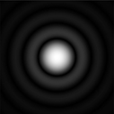
Figure 1. Example image of Airy disk pattern.

In this case, the image captures several orders of the Airy disk pattern with the full width of the image representing how the pattern would span 10.2 pixels (note that the center lobe probably spans around 2 pixels). For this setup, the image and scale options are used as shown below:

The same Airy Disk image can be used for systems with different aperture diameters and pixel pitches by simply changing the scale to reflect the scale of the pattern relative to the pixel size.

Example of using an image of Airy disk pattern for the PSF.

            "psf": {
              "image": "airy_disk.png",
              "scale": 10.2
            },

If you don’t have an image representing the PSF, then the Gaussian approximation for the center lobe of the Airy Disk (the ideal PSF for a clear, circular aperture) can be used instead. In the case the user simply provides the width at 1 sigma (in pixel sizes) for the pattern.

Example of using the built-in Gaussian approximationg for the PSF.

            "psf": {
              "width": 2.2
            },

Channel Options

In addition to the simple spectral description of the channel, the user can also include a set of advanced channel options that can be used to control how the output (either reflectance or radiance) is scaled to digital counts. This scaling is often handled as a post processing step, but the addition of it into the channel description means that the scaling can be randomized for each chip. The gain_range and bias_range define the ranges for a randomly generated gain and bias that are used to linearly scale the output (either reflectance or radiance) to digital counts (DCs) or other units. Unlike a post-processing approach that might use autoscaling on each image, this mechanism can more easily emulate situations where the system either saturates or underexposes the imagery.

When the scaling is applied, the output image data is still stored in a single-precision floating-point format. See the optional post-processing step if you want to convert the data to a different format.

Like all the random variables, setting the min and max for these gain and bias ranges to the same value results in a linear scale that is the same for every chip.

The (optional) noise_range allows the user to introduce simple additive noise to the output. Like most of the features in this plugin, the noise modeling has been simplified to this additive treatment because the plugin is aimed at producing datasets that emerge from higher levels in the product chain after several layers of processing (which typically includes noise reduction) have been applied. Hence, the modeling of low level mechanisms directly (Shot noise, read noise, etc.) is not the goal.

When using the channel scaling (via the gain and bias ranges), this noise is added after the scaling.

The example channel setup below shows a PAN channel with the optional scaling and noise. In this example, the gain and bias ranges were chosen to generate 8-bit imagery that sometimes saturated the 8-bit dynamic range (clipped).

Example of using the advanced channel options.

            "channellist": [
              {
                "name": "Pan",
                "maximum": 0.8,
                "minimum": 0.4,
                "gain_range": {
                  "minimum": 120000,
                  "maximum": 140000
                },
                "bias_range": {
                  "minimum": -600,
                  "maximum": -400
                },
                "noise_range": {
                  "minimum": 4,
                  "maximum": 10
                }
              }
            ],

When combined with the processing steps (see below), the linear scaling and noise can be used to directly generate chips in common formats (JPG, PNG, etc.) that include some noise and can be either saturated or underexposed.

Processing Options

The user has the option to specify a series of external processing tasks that will be executed at the completion of each chip. This can be used to convert the imagery to the desired output format, create truth masks, etc. Each processing "task" is composed of a message that will be displayed when the task executes and a command that contrains the external command to run as an array of strings representing the command itself and any arguments passed to it. The special string $$CHIP_BASENAME$$ represents the auto-generated base of the output file for that chip (e.g., chip_14).

The example below shows some processing steps for chips that contain 4 channels (pan, red, green and blue) and then some truth bands. In this example, the internal linear scaling feature (described above) was employed, so the radiance channels have already been scaled to an 8-bit value (0 → 255). Hence, the use of the DIRSIG image_tool to convert the image to PNG uses the --autoscale=none option. The input and output filenames for the command use the $$CHIP_BASENAME$$ string, which will be auto-replaced on-the-fly with the basename for the current image chip. The second task similar scales the RGB channels (band indexes 1, 2 and 3) to a PNG. The third task makes a PNG "target mask" image by auto-scaling band index 4, which corresponds to the object index truth in this example. Again, the $$CHIP_BASENAME$$ string is used to extract this truth to a separate file.

Example post-processing tasks to convert the image to PNG and to extract a mask for the target.

            "processing": [
              {
                "message": "Scaling Pan channel to PNG",
                "command": [
                  "image_tool", "convert",
                  "--autoscale=none", "--format=png", "--bands=0,0,0",
                  "--output_filename=$$CHIP_BASENAME$$_pan.png",
                  "$$CHIP_BASENAME$$.img"
                ]
              },
              {
                "message": "Scaling RGB channels to PNG",
                "command": [
                  "image_tool", "convert",
                  "--autoscale=none", "--format=png", "--bands=1,2,3",
                  "--output_filename=$$CHIP_BASENAME$$_rgb.png",
                  "$$CHIP_BASENAME$$.img"
                ]
              },
              {
                "message": "Making target mask PNG",
                "command": [
                  "image_tool", "convert",
                  "--autoscale=minmax", "--format=png", "--bands=4,4,4",
                  "--output_filename=$$CHIP_BASENAME$$_mask.png",
                  "$$CHIP_BASENAME$$.img"
                ]
              }
            ]

After each chip has completed, the full image cube (e.g., chip14.img), the scaled PAN image (chip14_pan.png), the scaled RGB image (chip14_rgb.png) and the mask image (chip14_mask.png) will be present.

Example output of DIRSIG when employing the processing steps above.

...
Starting chip 14 of 1000
    Image filename = 'chip2b.img'
    Target index = 56
    Tags = 'active', 'choppers', 'aircraft', 'ka27', 'korean'
    Location = -171.430450, -398.277191, -0.001000
    Offset = 2.451209, 2.969815, 0.000000
    Time = 100.35322 [seconds]
    GSD = 0.11076607 [meters]
    View angles = 23.469861875051965, 41.71914037499097 [degrees]
    View distance = 1000 [meters]
    Source angles = 35.05576149998286, 301.8145847050578 [degrees]
    Atmospheric conditions = 'mls_rural_10km'
Scaling the PAN channel to PNG
Scaling the RGB channels to PNG
Making target mask PNG
...

The example above uses the DIRSIG supplied image_tool utility, but processing steps can call any program, script, etc.

Time

Scenes that contain motion (moving objects) can be sampled as a function of time, which allows the moving objects to be imaged in different locations and/or orientations (as defined by their respective motion). The range of sample times is defined in the time_range section of the input. The minimum and maximum times are relative and in seconds.

View

The range of view directions for the camera is defined in the view section of the input. The zenith (declination from nadir) and azimuth (CW East of North) are supplied as minimum and maximum pairs. These angles are in degrees.

The optional offset_range will introduce a spatial offset of the target within the image. The range is used to generate a random XY offset to the selected targets location. The values are in meters. The default offset is 0 meters.

The optional distance_range will vary the "flying height" of the sensor. Given the orthographic projection of the chips, this parameter is normally irrelevant, but is useful to vary the amount of path radiance or extinction present in the chips when using the FourCurveAtmosphere model. The values are in meters. The default distance is 1000 meters.

Source

The direction of the source (sun) with relation to the target is defined in the view section of the input. The zenith (declination from nadir) and azimuth (CW East of North) are supplied as minimum and maximum pairs. This angles are in degrees.

Setup

The setup section of the file specifies the overall setup of the simulation to be performed, including the specification of which targets to sample, the number of images to be generated and the name of the file containing key label information.

target_tags: The list of tags used to select the targets in the scene to be imaged.
count: The number of image chips to generate.
random_seed: The random set of targets, view directions, source directions, etc. can be expected to change from simulation to simulation because the seed for the random number generator that drives these random parameters is different for each execution. If the user desires the ability to reproduce a specific simulation, then they can supply the random_seed variable to fix it so that it won’t change.
options: There are several options related to how the simulation runs. See below for more detail.
report_filename: The ASCII/text report that describes the target, view angles, illumination angles, GSD, etc. for each image chip is written to the filename provided by this variable.

Options

The following options control how the simulation is performed.

hide_others: This option will cause the simulation to hide all the other targets in the selection set while the chip for a given target is being generated. In the example above the selection set includes anything that has the tags "box" and "sphere". Therefore each chip will be centered on a "box" or sphere". With this option included, all other "box" and "sphere" objects will be hidden except for the one being imaged. Note that "cylinders" (not included in the example tag set) will not be a chip target or be hidden when imaging any of the "box" or "sphere" targets.
with_and_without: This option will cause the simulation to produce A/B image pairs with and without the current target present. If there are N chips requested (see the count variable in the setup), the resulting images will be named chip0a.img (contains the target) and chip0b.img (same parameters, but without the target).
rerun_from_report: This option allows the user to reproduce a set of images using the output label report (see the report_filename variable in the setup) from a previous simulation. When using this mode, rather than choose a random target, random view, etc. it will use the parameters (target index, time, GSD, source angles, etc.) from the report file. Note that if the scene changes (specifically if, new targets are added), then the output image set will be different.
make_meta: This option will create a small meta-data file for each chip that contains meta data for that chip in an easily parsable JSON format (for example, chip10.img will have a file named chip10.meta).

The with_and_without and rerun_from_report options cannot be combined at this time.

Output

Illumination and output units

When using the FourCurveAtmosphere model, the output units are radiance in Watts/cm² sr.

When not using the FourCurveAtmosphere model, the direct/diffuse illumination partitioning is fixed at 80% and 20%, respectively. The total hemispherical irradiance is currently Pi, which results in output images that have units of total reflectance. This allows the end user to easy calibrate the images into whatever units space they desire.

Image format

The output image is an binary/text ENVI image data/header file pair. The image data is single-precision floating-point and the bands are written in a band-interleaved by pixel (BIP) order. The first N bands in the image contain the channels defined in the sensor description. The remaining bands contain the truth data requested.

Meta Data Files

If the optional meta-data files are generated (enabled via the make_meta option), the a small JSON file is created for each chip image. This file contains the values for all the key variables for the chip.

An example meta-data JSON file.

{
    "image_filename" : "chip01.img",
    "image_size" : [180,180],
    "target_index" : 57,
    "gsd" : 0.281232,
    "time" : 102.417,
    "view_zenith" : 0.24056,
    "view_azimuth" : 5.71626,
    "view_distance" : 1000,
    "source_zenith" : 0.276679,
    "source_azimuth" : 4.24691,
    "atm_conditions" : "mls_rural_15km_dis8.tp5",
    "tags" : ["aircraft","ka27","choppers","idle","korean"]
}

Usage

To use the ChipMaker plugin in DIRSIG5, the user must use the newer JSON formatted simulation input file (referred to a JSIM file with a .jsim file extension). At this time, these files are hand-crafted (no graphical editor is available).

The JSON configuration for the plugin can be stored inside the plugin’s respective inputs object, or in a separate JSON file via the input_filename variable:

An example of a ChipMaker setup using an internal JSON description.

[{
  "scene_list" : [
    { "inputs" : "./demo.scene" }
  ],
  "plugin_list" : [
    {
      "name" : "ChipMaker",
      "inputs" : {
        "atmosphere" : {
          "database" : "./my_atm_db.hdf",
          "conditions" : [
            "nice_conditions", "yucky_conditions", "ok_conditions"
          ]
        },
        "camera" : {
          "image_size" : {
            "x" : 128,
            "y" : 128
          },
          ...
        },
        ...
        "setup" : {
          "random_seed" : 54321,
          "target_tags" : [ "box", "sphere" ],
          "options" : [ "with_and_without" ],
          "count" : 100,
          "report_filename" : "labels.txt"
        }
      }
    }
  ]
}]

An example of a ChipMaker setup using an external JSON description.

[{
  "scene_list" : [
    { "inputs" : "./demo.scene" }
  ],
  "plugin_list" : [
    {
      "name" : "ChipMaker",
      "inputs" : {
        "input_filename" : "./chips.json"
      }
    }
  ]
}]

The ChipMaker2 Demo

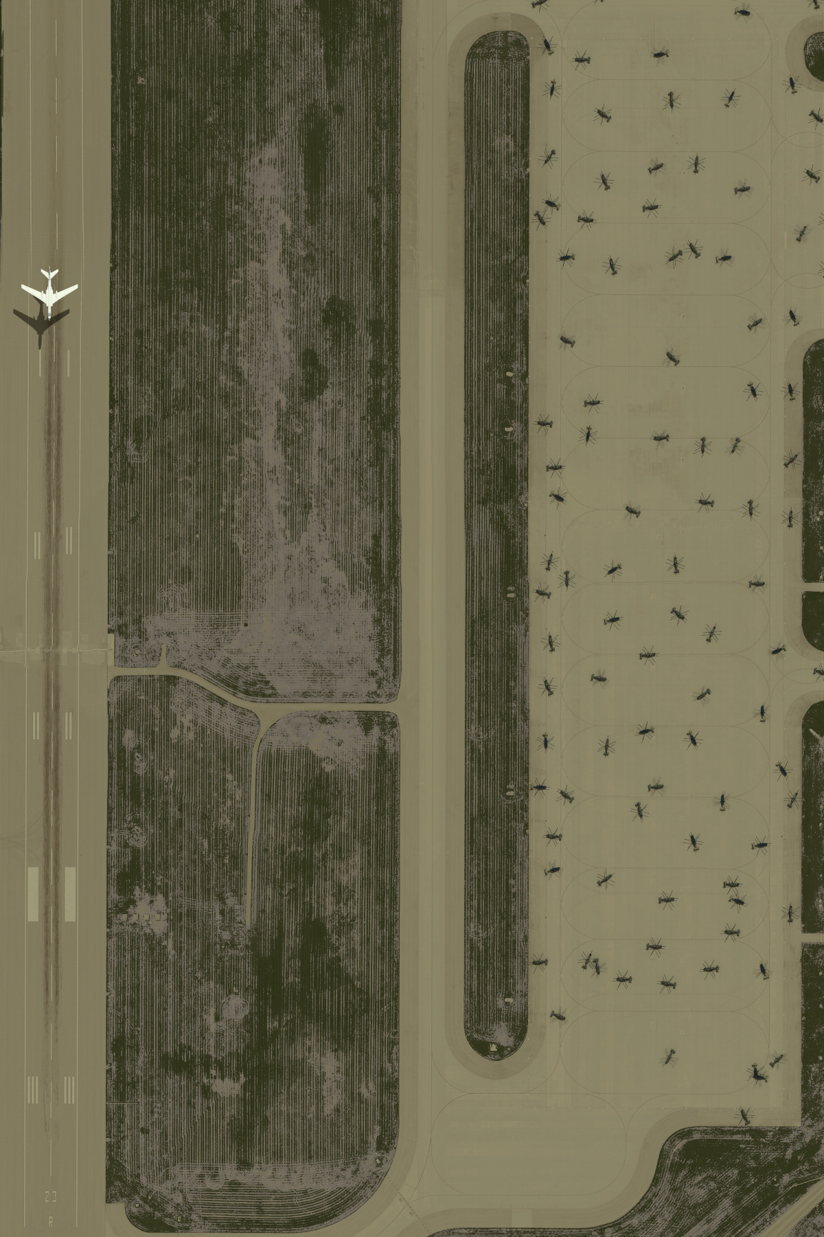
The ChipMaker2 contains a working example of this plugin. The demo contains a scene that includes 100s of helicopters and a few planes. There are 3 material variants of the same helicopter (Indian, Korean and Russian schemes) and for each of those there are "idle" (rotor is not spinning) and "active" (rotors are spinning) variants. The plane is defined with a dynamic instance that has it landing on the runway. The image below shows what the scene looks like at a given time.

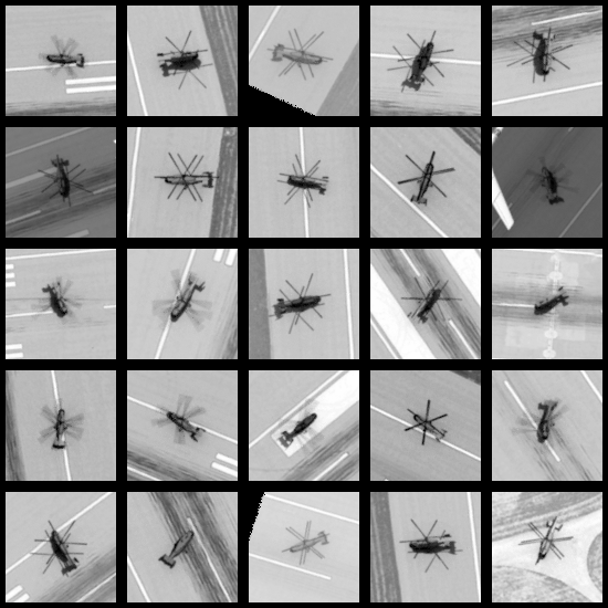
Figure 2. Overhead view of the ChipMaker2 demo scene.

To get chips of the helicopters there are many tags to choose from. The general "choppers" tag will get all the helicopters. The "idle" tag will get all the idle helicopters regardless of country scheme. The "russian" tag will get the "idle" and "active" helicopters with the Russian material scheme. The image below shows a set of chips just using the general "chopper" tag:

Figure 3. A chipset using the "choppers" tag.

For the helicopters, the rotors are spinning but they all have static instances (each helicopter is fixed at it’s position). Use of the time_range would mean each chip looks at the object at a different time within the time range. For the helicopters, that would mean seeing the rotors in different positions. Since the plane is moving (it has a dynamic instance), the time_range can be employed with greater effect. 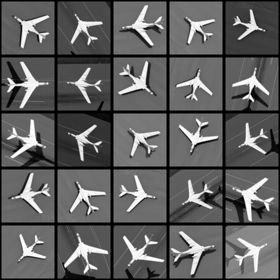In this case, it will find the plane in different locations during the time window. The chip set below is all of the same plane, but using a time range that images it well above the runway on approach through when it has landed (and everywhere in between):

Figure 4. A chipset using the "planes" tag.