To maximize the flexibility in modeling end-to-end LIDAR systems, a full simulation is divided into two, discrete stages. Stage 1 is the "Radiometric Simulation" that (for each pulse) computes the temporal flux received by each pixel during a user-specified listening window. That result is then input into Stage 2, or the "Detector Model and Product Generation" stage, where the output of Stage 1 is coupled with a separate, back-end detection model to convert the temporal photon arrival times into common data products (e.g. geo-located point clouds):
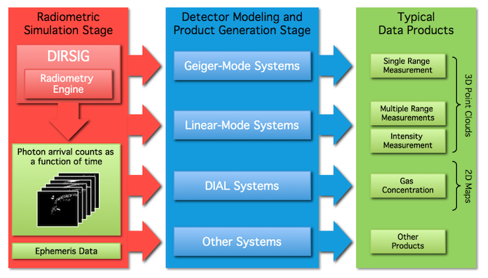
The DIRSIG model is distributed with a generalized tool for the detection and product generation stage that is capable of modeling simple GmAPD systems, LmADP systems and hybrid photon-counting systems (like that employed in ICESat-2). A more detailed explanation of that tool can be found in the LIDAR Modality Handbook. This document is focused on the advanced GmAPD modeling capabilities that have been developed for use with the DIRSIG model.
|
|
This advanced model was made available in DIRSIG 4.7, and it focuses on modeling specific aspects of GmAPD systems. However, this tool requires a great deal of engineering data (that is not generally available) in order to be used effectively. For most users, the basic GmAPD model described in LIDAR Modality Handbook is sufficient. |
Overview
The flowchart below highlights the various components components of the advanced GmAPD detector modeling capability:
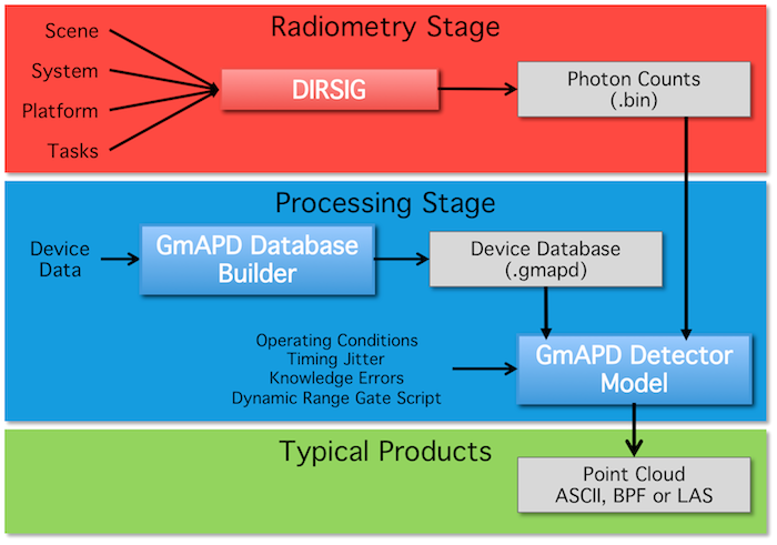
The top tier (red) represents conventional DIRSIG model and it’s role in the generation of per-pixel arrival photon count waveforms on a pulse-by-pulse basis. The middle tier (blue) represents the tools providing the advanced GmAPD detector modeling capability. This tier is primarily composed of the GmAPD Database Builder and the GmAPD Detector Model tools, which will be the focus of the rest of this document. The bottom tier (green) represents the output data products, which are Level-1 points clouds in various formats.
GmAPD Database Builder
The primary function of the GmAPD Database Builder tool is to create databases that characterize the performance characteristics of a GmAPD array. This database will be used by the GmAPD Detector Model to determine time-of-flight firings in response to arriving photon flux waveforms. The GmAPD database contains the following properties as a function of device operating temperature and applied bias voltage:
-
The photon detection efficiency (PDE)
-
This captures the overall efficiency of the device including the (optional) lenslet transmission, quantum efficiency and avalanche probability.
-
-
The dark count rate (DCR)
-
This captures the rate at which spontaneous avalanches occur in the absence of input photons.
-
-
The pixel cross-talk
-
This captures the likelihood that an avalanche in one pixel will cause an avalanche in one or more neighboring pixels.
-
The PDE and DCR data is provided on a per-pixel basis for each temperature/bias profile. The pixel cross-talk is array-averaged for each temperature/bias profile.
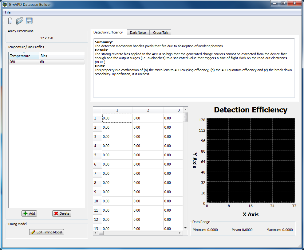
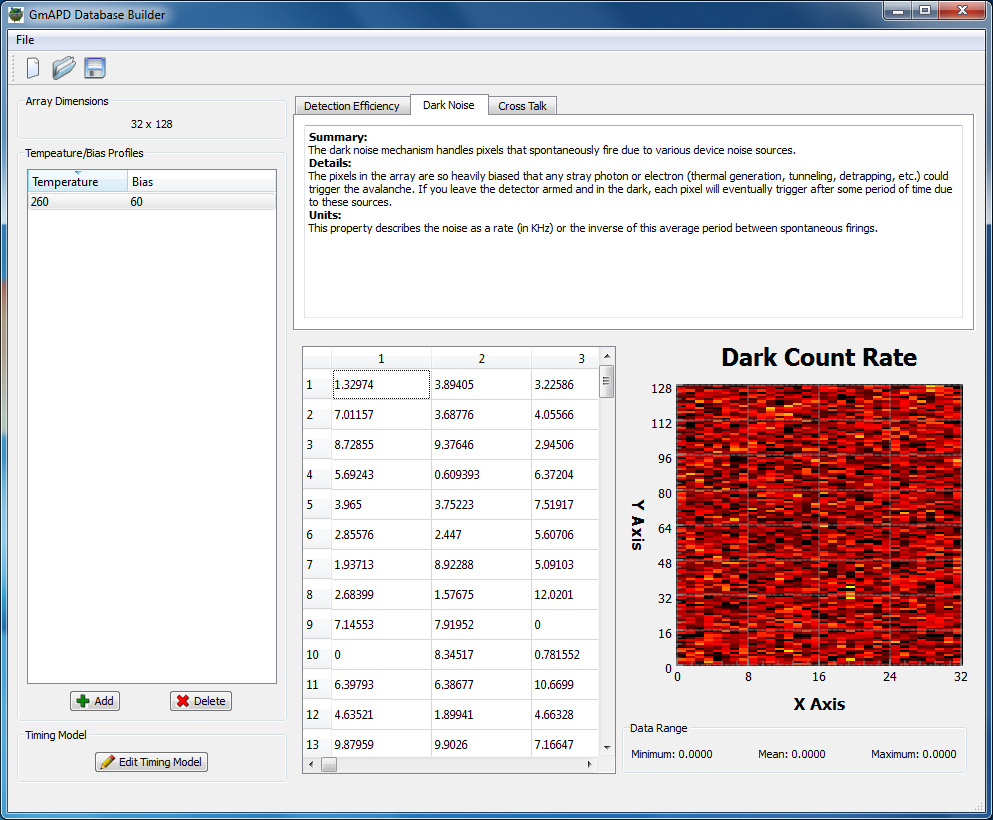
The tool can be launched via the GmAPD Database Builder item in the Lidar Tools sub-menu of the Tools menu of the DIRSIG Simulation Editor. The left-hand side of the tool displays the list of available temperature and bias profiles contained in the database. By selecting one of these profile items, the data associated with that profile will be loaded into the right-hand side of the tool for editing and visualization. The table area allows the user to view and edit the per-pixel values for the PDE and DCR data. The plot area allows the user to visualize these per-pixel values.
Creating a new database
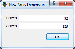
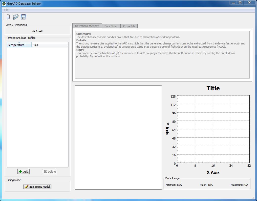
To create a new database, select the New item from the File menu or click the New icon in the toolbar. This will pop-up a dialog box that asks the user to define the size of the array that will be characterized. In the following example, we create a database for a 32 x 128 array:
Creating a new Temperature/Bias profile
The first step in making a minimal GmAPD device database is to define at least one temperature/bias profile. To add a new profile, click the Add button below the Temperature/Bias Profiles list on the left-hand side of the tool.
This will pop-up a dialog asking the user to define the temperature and bias for this profile:
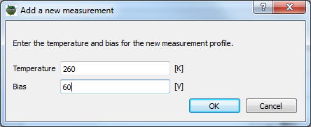
In this example we are going to import data for a device operating
at a 265.0 Kelvin and a bias voltage of 60.0 volts.
|
|
Although the actual bias voltage may be negative (for example, -60.0 volts) the magnitude is the key piece of information and the convention here has been to use positive values. |
Select the new profile by clicking on the one item in the Temperature/Bias
Profiles list on the left-hand side of the tool. The right-hand side of
the tool will now be enabled so that you can browse the PDE, DCR and
cross-talk data associated with this temperature/bias setting. The
default values in a new profile for the PDE, DCR and cross-talk are
all 0.0.
|
|
The ability to create and manage multiple temperature and bias profiles allows the user to model the system performance characteristics under different operating conditions. In many cases involving specifications from a manufacturer, these operating conditions are not known. In those cases the user should create a single profile with arbitrary temperature and bias values. When only a single profile is available, it will be the default profile (always used) and the temperature and bias values supplied as operating conditions are irrelevant. |
Adding PDE and DCR data into a profile
The next step is adding non-zero values for the PDE, DCR and cross-talk. The units for the data for the PDE and DCR are:
-
The PDE values are fractional values between 0 and 1.
-
The DCR values are in units of kHz and not Hz.
The PDE and DCR data support per-pixel values, which can be set using a variety of methods.
Manual entry of PDE and DCR data
Any pixel in either the PDE or DCR can be manually edit in the table area.
This allows the user to manually tweak a single pixel to make a "hot pixel"
by increasing the DCR or to create a "dead pixel" by setting the PDE to 0.
Filling the PDE and DCR data with values
If the user right-mouse clicks inside the table area, a menu will pop-up containing a Fill item. Selecting this item will allow the user to "fill" the table with values created from a user-supplied mean and standard deviation.
Importing per-pixel PDE and DCR data
If the user has access to a per-pixel map of the PDE or DCR, then that data can be imported into a profile. The right-mouse click menu in the table area includes a Import item that starts this process. The user will then be prompted to specify an ASCII/Text file that contains the PDE or DCR values for each pixel. The format of the file is extremely simple, consisting of a stream of whitespace delimited values. The values can appear on individual lines, a line for each row in the array or one (very long line).
|
|
"Whitespace delimited" means any number of "whitespace" characters can appear between the values. These include spaces, tabs and newlines. It does not include commas, colons, etc. |
|
|
The order of the values is "row major", which means the values in the file start with the first row, first column and then proceed through all the columns in that row before starting on the next row. |
Below is an example ASCII/Text file that can be imported:
0.22075
0.19132
0.26299
...
[lines deleted for documentation purposes]
...
0.23589
0.28769
Where the value 0.22075 corresponds to pixel (0,0), the value
0.19132 corresponds to pixel (0,1) and 0.28769 corresponds
to pixel (31,127) in a 32 x 128 array.
Note that the simple format of the file does not facilitate much error checking by the software. If the file does not contain the correct number of values for the array size defined, then an error will be issued.
|
|
Always check the values of a few pixels after you import data to insure that the data was correctly read in. |
Adding cross-talk data into a profile
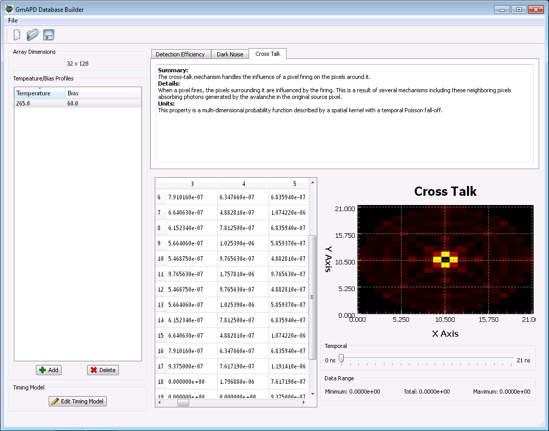
Unlike the 2D (pixel row and column) PDE and DCR maps for a given profile, the cross-talk is characterized by a 3D map that defines the probability of neighboring pixels firing due to a fire event in a given pixel. This 3D probability kernel is 21 pixels x 21 pixels x 21 time bins.
Importing 1D measured cross-talk data
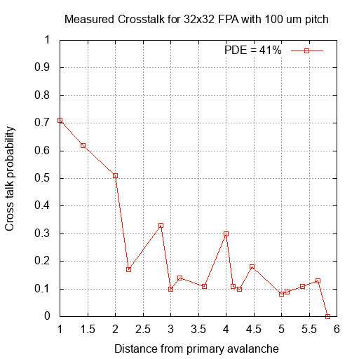
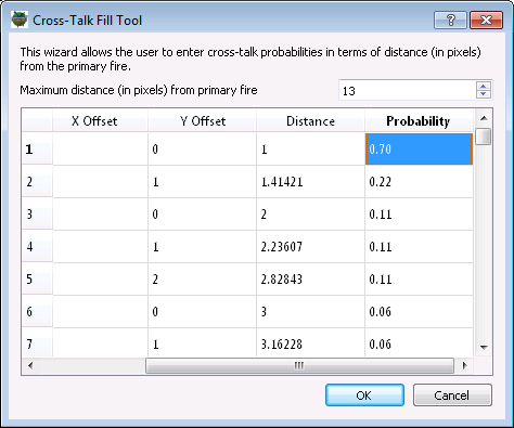
If the user has access to a 1D radially-symmetric, temporally-summed cross-talk, then that data can be imported into a profile. This type of data has been published by some commercial GmAPD manufacturers (see plot below). The right-mouse click menu in the table area includes a Fill item that starts this process. The 1D cross-talk fill wizard provides an interface to specify total (time summed) cross-talk probabilities as a function of radial pixel distance from the originating avalanche event. The wizard allows the user to specify the maximum radial distance from the primary avalanche for which probabilities are known. The wizard will then generate a table of relative offsets to a neighboring pixel, the radial distance to that neighboring pixel and a probability of a subsequent event within that neighboring pixel. The user must fill in the probability using the other columns as a guide. Most published plots are in terms of the radial distance, but for some reason don’t include values for all pixel offsets within the maximum radius. In cases where a data point is not explicitly provided for a given distance, interpolating from known distances is recommended.
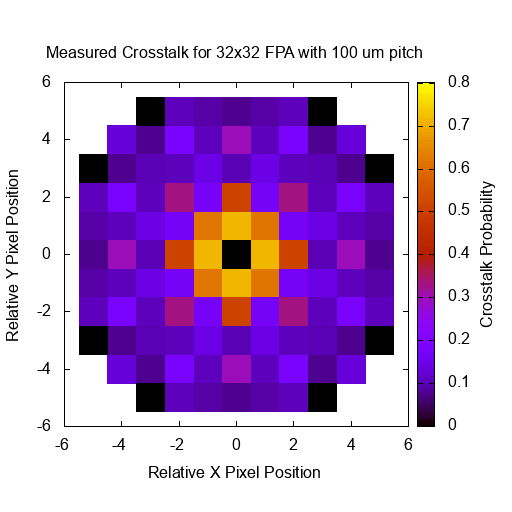
This 1D radial profile is then used to construct a 2D spatial map (see plot below). Pixel distances beyond those defined by the profile are assumed to be 0. The time dimension of the 3D cross-talk cube is modeled as an exponential decay in the 2D map.
Importing 3D measured cross-talk data
If the user has access to a 3D spatial x spatial x time kernel for the cross-talk, then that data can be imported into a profile. The right-mouse click menu in the table area includes a Import item that starts this process. The user will then be prompted to specify an ASCII/Text file that contains the PDE or DCR values for each pixel. The format of the file is extremely simple, consisting of a stream of whitespace delimited values. The values can appear on individual lines, a line for each row in the array or one (very long line).
|
|
The order of the values is "time sequential, row major", which means the values in the file start with the first time slice of the cube and with the first row, first column and then proceed through all the columns in that row before starting on the next row. After all the rows in that time slice are read, the next time slice is read. |
Below is an example file containing 3D cross-talk data:
0.00033854 0.00034947 0.00041432 ... 0.00036731
0.00036088 0.00035864 0.00042960 ... 0.00031368
...
[lines deleted for documentation purposes]
...
1.7195e-005 3.5678e-005 2.9185e-005 ... 2.9022e-005
The first 21 lines in the file represent the first 21 x 21 time slice. Each of these lines has 21 values corresponding to the 21 columns in this time slab. The next 21 lines contain the next 21 x 21 time slice, and that continues until all 9,261 values are read.
|
|
Since the input values only need to be whitespace delimited, this data could also have been formatted as 21 single lines containing 441 values, where each line would then represent a single 21 x 21 slice in the 3D probability cube. This data could also have been formatted as a single line containing 9,261 values or 9,261 lines containing a single value. The important thing is the order of the values and not how many lines the data is formatted into. |
Scaling 3D cross-talk data
Some manufactures publish a total cumulative cross-talk probability, which incorporates the probably of any pixel triggering as a result of primary avalanche. This includes secondary pixels that trigger directly from the primary avalanche as well as pixels that trigger due to those secondary triggers, etc. Hence, it captures the probability of a chains of cross-talk events.
The database tool allows the user to scale whatever cross-talk data has been loaded into the profile. This tool is accessed via the Scale item in the right-click menu for the cross-talk data table. It will open a dialog window that displays what the current total cross-talk probability is and allows the user specify what they would like to change it to. The scaling process uniformly scales the 3D cross-talk to achieve the desired value.
GmAPD Detector Model
Technical Overview
The GmAPD Detector Model tool encapsulates two primary roles:
-
Modeling when the GmAPD device will fire in response to an incident photon arrival waveform and noise sources. This results in a time-of-flight measurement for each pixel in the array for each pulse.
-
The generation of a point in the output point cloud by employing the measured time-of-flight, the atmospheric properties, the current position and orientation of the platform and the current platform-relative pointing.
The details of these two roles are discussed in the following sections.
Detection
A detailed description of the detection model implementation is beyond the scope of this document. But the algorithm includes the following aspects:
-
The inclusion of photon detection efficiency and dark count noise using an approach inspired by the work of Flouche and O’Brien at MIT Lincoln Laboratory.
-
The inclusion of "early fire" events, or the firing of pixels in the first time bin due to photo-electrons that accumulate while the device is not armed.
-
The inclusion of pixel "cross-talk", or the firing of neighboring pixels due to photons generated when a pixel fires.
-
Support for temperature and bias voltage dependent per-pixel PDE, per-pixel DCR and array uniform cross-talk.
-
Support for vernier bit timing non-uniformities, which lead to irregularly structured ranges.
Point Generation
The result of the detection process is a time-of-flight measurement for each pixel. The point generation aspect of the tool determines where to create a point in the point cloud based on a given time-of-flight measurement. The idealized version of the process involves the following steps:
-
The time-of-flight is converted to a total distance traveled using a nominal speed of light.
-
The total distance is halved to determine the range to the object responsible for the return.
-
The platform orientation and platform-relative pointing is used to figure out where the return is relative to the platform location.
-
The point is translated from a position relative to the platform to an absolute location using the platform location.
With the idealized point generation process described, the tool supports the following advanced options to address many real-world limitations that can render the idealized approach invalid.
-
Rather than assume the speed of light is constant, the tool allows a vertically structured atmospheric description to be supplied.
-
The model will then compute the bent path to the return.
-
-
Rather than use precise knowledge of the platform location, platform orientation, platform-relative pointing and lens distortion, the model allows the user to introduce various "knowledge errors"
-
The user can temporally average, quantize and add noise to the platform and scanner ephemeris values.
-
The output of the point generation process is a Level-1 point cloud. Currently the user can choose from four different output point cloud file formats:
-
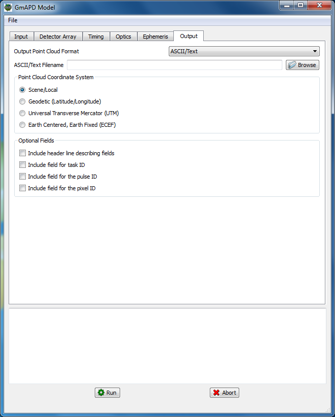
ASCII/Text Format
-
Point locations in either Scene ENU, Latitude/Longitude, Universal Transverse Mercator (UTM) or Earth-Centered, Earth-Fixed (ECEF).
-
Optional fields (columns) for pixel index, pulse (frame) index and task index.
-
-
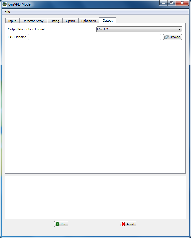
LAS 1.2 Format
-
Minimally formatted file with no point meta-data.
-
-
BPF Version 2 Format
-
End-of-gate (EOG) points are always included.
-
Every point includes the pixel index, pulse (frame) index and end-of-gate flag.
-
-
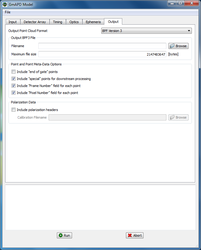
BPF Version 3 Format
-
User option to include "special points" (per-pulse platform location and FPA field-of-view frustum).
-
User option to include the pixel index.
-
User option to include the pulse (frame) index.
-
User option to include end-of-gate (EOG) points.
-
Tool Overview
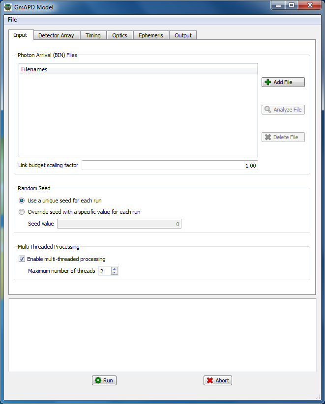
The tool can be launched via the GmAPD Detector Model item in the Lidar Tools sub-menu in the Tools menu of the DIRSIG Simulation Editor.
Input Radiometry (BIN) Files
The Input tab of the tool allows the user to specify one or more input photon arrival count (BIN) files that were calculated by the DIRSIG model during the Radiometric Simulation stage.
|
|
If more than one BIN is specified, the resulting points will be merged into the single output point cloud file. |
Files to be processed are added to the list by clicking the Add button and browsing to the desired file. Files to be processed can be removed from the list by selecting the file in the list and clicking the Delete button.
|
|
The Analyze button will run the BIN file analysis tool, which outputs various headers embedded in the BIN file and computes useful per-pulse statistics. |
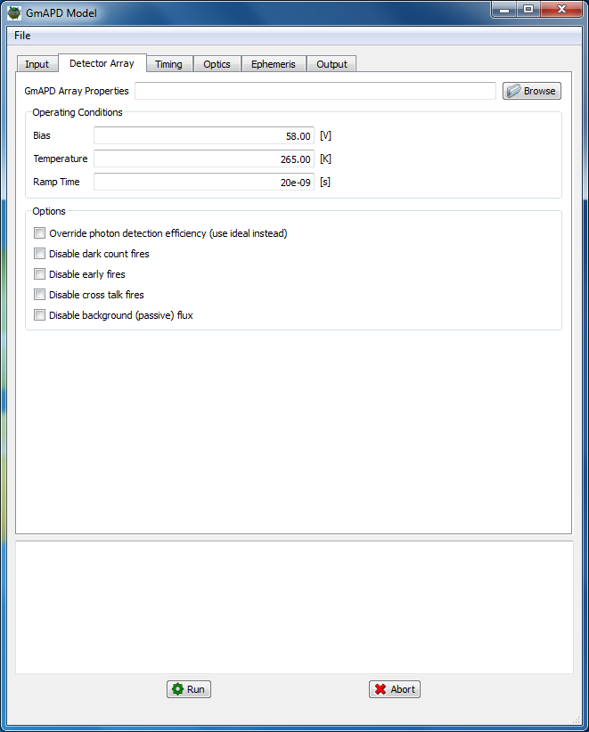
Array Operating Conditions
The operational conditions of the Geiger-mode array and detection modeling options are specified on the Detector Array tab. This includes:
-
A GmAPD device database created with the GmAPD Database Builder tool.
-
The desired array operating conditions, including the temperature, bias voltage and ramp time.
-
A variety of modeling options are also available:
-
The option to override the per-pixel PDE with an array-wide, ideal (unity) PDE.
-
The option to override the per-pixel DCR with an array-wide, ideal (zero) DCR.
-
The option to disable "early fire" triggers.
-
The option to disable cross-talk generated triggers.
-
|
|
The Ramp Time parameter drives the "early fire" mechanism. The longer the ramp time, the greater the probability of an early fire event. |
|
|
The "early fire" mechanism can be disabled by either the explicit disable button, or by setting the Ramp Time to 0 seconds. |
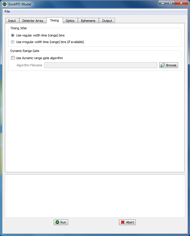
Timing and Vernier Bit Effects
The Timing tab provides the user access to the toggle the use irregularly sized vernier bit time bin data in the GmAPD device database (if available).
This tab also allows the user to supply a dynamic range gate script. These range gate scripts look at the fires from the previous pulse and set the new open and close for the current pulse. The way to use these scripts is to run DIRSIG with a much larger listening window than you want to finish with. For example, if you want to model a 2 microsecond range gate that can slide +/- 5 microseconds, then you need to model a 12 microsecond gate in DIRSIG and then let the dynamic range gate scripts control which 2 microsecond portion of that 12 microsecond range gate is used.
The model is distributed with two example scripts, but the user is free to create their own:
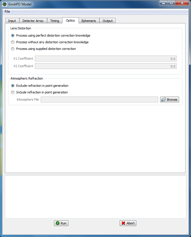
Optics and Atmospheric Refraction
The Optics tab allows the user to control various knowledge aspects of the optical path inside the receiver and the atmosphere in the scene.
The Lens Distortion options include:
-
Generate points with precise knowledge of the receiver optics distortions, or
-
Generate points assuming the receiver optics are perfect (distortion free), or
-
If the actual receiver was not ideal, then this is a source of knowledge error.
-
-
Generate points by supplying the receiver optics distortion coefficients
-
If these coefficients do not match the actual receiver, then this is a source of knowledge error.
-
The Atmospheric Refraction allows the user to:
-
Assume a uniform atmosphere with a nominal index of refraction, or
-
Provide a vertical description of the atmosphere that will drive bent path calculations
-
If the supplied atmospheric description does not match the atmospheric description used in the DIRSIG Radiometric Simulation, then this is a source of knowledge error.
-
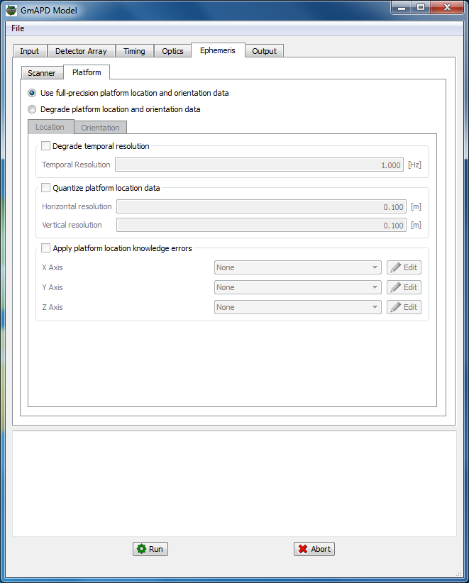
Ephemeris and Knowledge Errors
The Ephemeris tab allows the user to introduce various sources of knowledge error to the location of the platform, orientation of the platform and platform relative pointing (scanning). The BIN file contains precise values for these three components on a per-pulse basis, allowing the model to simulate system with perfect knowledge. To create a more realistic simulation, the user can introduce various source of knowledge error. For each of these three components, the user can:
-
Temporally degrade the data, which simulates the limited sampling frequency of most GPS and IMU systems.
-
Quantize the resolution of the data, which simulates the limited precision of the most GPS and IMU systems.
-
Introduce temporally uncorrelated and correlated (frequency spectrum driven) errors to the measured data.
Output Point Cloud Format
The Output tab is where the user specifies the format of the output point cloud file. Each output format has a unique set of options related to it.
Tutorials
Importing Commercial Specifications
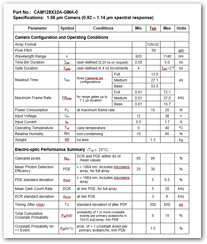
For this example, we will be incorporating the published performance specifications for a commercially available 128x32 GmAPD camera produced by Princeton Lightwave, Inc. (PLI).
|
|
The PLI camera specifications captured here for this example are from October 2015. Please consult the manufacturer’s website for up-to-date specifications. |
The key performance metrics of interest here are the Photon Detection Efficiency (PDE) and Dark Count Rate (DCR) values:
| PDE | DCR | |
|---|---|---|
Mean (typical) |
30% |
5 kHz |
Standard deviation (typical) |
5% |
3 kHz |
Creating a new database
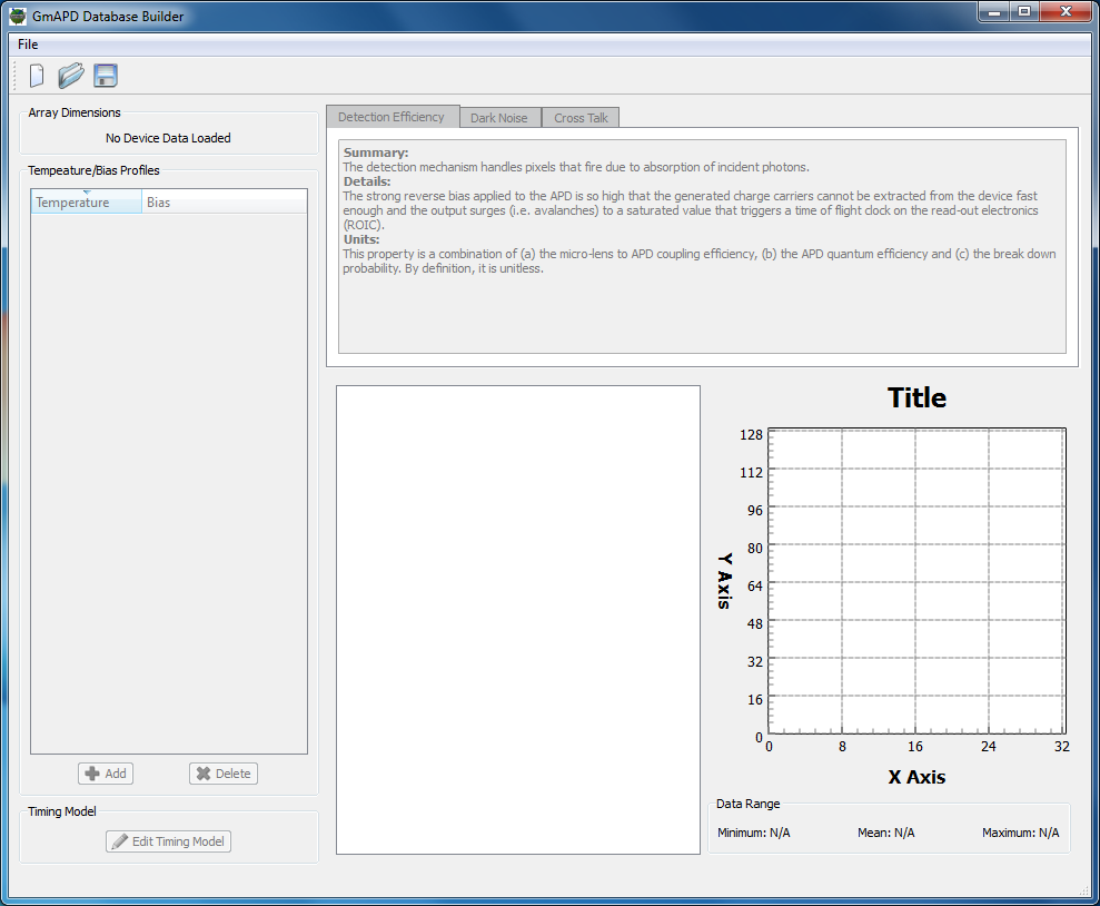
To create a new GmAPD database, start the GmAPD Database Builder tool. The tool will open without a database loaded:
First, we need to specify the size of the array. Click the New item in the File menu or the New icon and set the array size to 32 x 128 in the dialog:
Creating a default profile
At this point the tool is ready to start having temperature and bias profile data imported. The PLI spec sheet doesn’t provide these internal operating parameters, so we will arbitrarily use 260 K and 60 V.
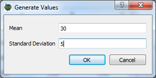
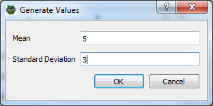
Filling the PDE values
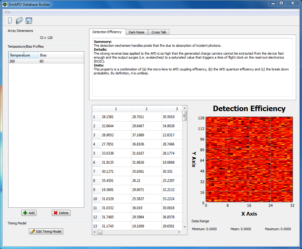
According to the spec sheet, the PDE values have a mean of 30% and a standard deviation of 5%. These values can be utilized by using the Fill option available on the right-click menu when over the PDE data table on the Detection Efficiency tab:
After clicking the OK button on the fill dialog, the data table and visualization will be filled with generated values.
Filling the DCR values
According to the spec sheet, the DCR values have a mean of 5 kHz nd a standard deviation of 3 kHz. These values can be utilized by using the Fill option available on the right-click menu when over the DCR data table on the Dark Noise tab:
After clicking the OK button on the fill dialog, a second dialog will probably appear:
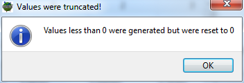
This warning appears because a mean of 5 and a standard deviation of 3 results in generating some values less than 0. Since a negative dark count rate doesn’t make physical sense, the tool will reset these negative values to zero. After clicking OK on the warning dialog, the data table and visualization will be filled with generated values.
Addressing the Cross Talk
Although the PLI spec sheet provides ensemble cross talk performance metrics (the number of subsequent events that can result from a primary event) it doesn’t capture the spatially and temporal distribution of these events. For example, the highest probability of cross talk is usually in one of the neighboring pixels during one of the next few range bins. Therefore, we need additional information that captures the spatial and temporal distribution of the cross-talk. In 2011, PLI published a paper at the OSA "Applications of Lasers for Sensing and Free Space Communications" conference in Toronto, CA. Figure 4 in that paper contained 1D plots of the cross-talk probability as a function of radial distance from the primary avalanche for a PDE of 35%. These published plots were manually digitized to create the 1D radial cross-talk profile below:
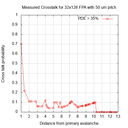
The 1D data was then imported using the Fill tool in the right-click menu for the cross-talk data table using a maximum radius of 13:
Typing in all the values can be a tedius process, so the resulting 3D
cross-talk data is provided in the lib/data/gmapd folder within the
DIRSIG installation. It can be loaded using the Import item in the
right-click menu for the cross-talk data table. The screenshot below
shows the resulting 2D spatial pattern produced by the 1D profile:
The PLI spec sheet says that the total cumulative cross-talk probability is 8%. To insure that our import cross-talk matches that total value, use the Scale tool in the right-click menu for the cross-talk data table. The tool will calculate the total value for the data currently in the table and then let you specify the value you would like it to be. In this case we want to insure it is 0.08.

Note that the initial difference in values is likely due to the published 1D profiles already containing the total probability, but the tool is interpreting the imported data as a single event probability.
Demonstrations
In addition to the LIDAR demos highlighted in the LIDAR Modality Handbook, there is an additional set of demos that are specific to using the Advanced GmAPD model.
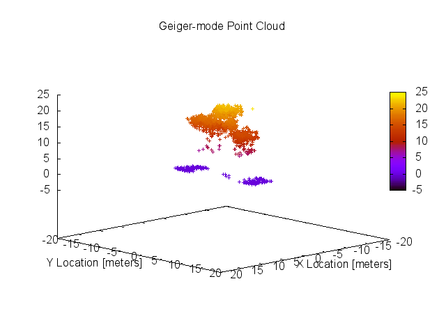
Single-Pulse
The LidarStatic2 demo shoots a single pulse onto a tree and receives that pulse onto a 32 x 128 array using the PLI specifications outlined in the tutorial:
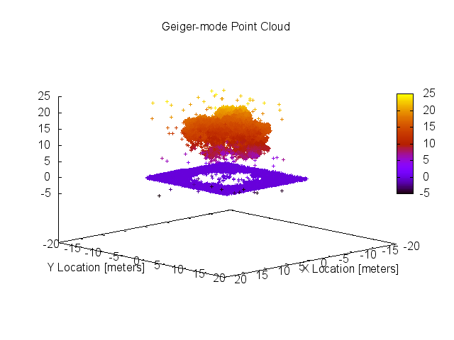
Multi-Pulse Scanning
The LidarWhisk2 demo shoots a series of 40 overlapping pulses while scanning a 32 x 128 array in the across-track dimension.
References
-
O’Brien, M. and D. Fouche, "Simulation of 3D laser radar systems," Lincoln Laboratory Journal, Vol. 15, No. 1, pp. 37-60 (2005), https://www.ll.mit.edu/publications/journal/pdf/vol15_no1/15_1simulation.pdf
-
Itzler, M. A., Entwistle, M., Owens, M., Patel, K., Jiang, X., Slomkowski, K., and Rangwala, S., "Geiger-mode Avalanche Photodiode Focal Plane Arrays for 3D LIDAR Imaging", Applications of Lasers for Sensing and Free Space Communications Technical Digest, OSA, Toronto, Ontario, Canada, (2011), https://doi.org/10.1364/LSC.2011.LThA3