Introduction
Most of the commercial rendering packages used for TV and movie production focus on producing visible images with red, green and blue (RGB) channels. In contrast, the DIRSIG model was developed for simulating remote sensing platforms, which generally image natural scenes and many different wavelengths. In order to support systems engineering of complex remote sensing platforms, the radiometry framework in the DIRSIG model must be able to simulate 10s, 100s and even thousands of wavelengths. It must also be able to account for thermal (self) emission and active illumination (for example, laser radar).
Driven by a the focus on remote sensing platforms and natural scenes, the following approaches are employed:
-
Most natural scenes contain surfaces that are generally low reflectance (overall reflectances less than 20%) and diffuse (nearly Lambertian). Under these conditions, hierarchical ray tracing may be more efficient than pure path tracing.
-
Most materials do not have BRDFs that vary rapidly with wavelength (blue is not very specular while red is very diffuse). Therefore, we can utilize spectrally averaged BRDFs to drive importance sampling. Note that although spectrally averaged BRDFs are used to drive where to sample, the spectrally varying BRDF is always used to fold in the radiometric contribution for a given sample.
-
Different surfaces (or volumes) can have different materials, which can have different optical properties. Specialized algorithms for solving surface (or volume) leaving fluxes can be more efficient than a generalized approach for all kinds of materials.
In DIRSIG4, we call these specific algorithms radiometry solvers and they compute the surface (or volume) leaving radiance for a spectral range during a single calculation.
Radiometry Solvers
The radiometry solvers within the DIRSIG4 model are computational objects that are responsible for predicting the radiational flux from a specific radiational element under a supplied set of conditions (e.g the date/time, view angles and solid angle). A "radiational element" might be a surface such as a leaf on a tree, the hood of a car, the roof of a building, or a sidewalk. A "radiational element" might also be a volume such as a cloud, water, etc. In operation, the solver is called during the stepwise radiative transfer to compute the flux contribution along the path and (potentially) the transmission through the element. The radiometry subsystem uses these radiometry computation engines in an effort to make the model very flexible. At the present time, the DIRSIG4 model includes a handful of specialized radiometry solvers that utilize different approaches to computing the radiation contributions. For example, there are radiometry solvers that are specifically designed to model gas volumes and others for solid surfaces. For a solid surface, different radiometry solvers might utilize a different incident illumination algorithm or a different sampling algorithm to compute the incident illumination.
-
The radiometry solvers are primarily an algorithm object.
-
However, as an object, each instance of the same algorithm can be configured differently and has the ability to store data as well.
-
-
There is a unique instance of the solver object associated with each material it is assigned to.
-
That means each instance of a solver can be optimized at run time for the specific material it is assigned to.
-
-
Each solver has access to the material it is associated with (its "parent" material), through which it can access the surface optical properties.
-
The SurfaceProperties object provides a proxy interface to the surface optical properties (e.g. reflectance, emissivity, etc.).
-
The BulkProperties object provides a proxy interface to the bulk or volume optical properties (e.g. scattering, extinction, etc.).
-
By making the radiometry solvers objects, the user is allowed to change the radiometry solver associated with any radiational element at run-time. This flexibility allows the user to experiment with different approaches to modeling a specific radiational element. In addition, it allows the developers to create new radiometry solvers and test them without impacting the rest of the user base.
Each solver object has two primary functions that are called during the course of a simulation:
-
The
init()function is called at the start of the simulation-
This allows each solver instance to optimize internal parameters or data structures for the material it is assigned to.
-
-
The
compute()function is called to compute the leaving radiance for the specific conditions.-
Even though a given instance of a solver might be attached to a material called "glass", each call to the
compute()function will be for glass in a different location of the scene, at a different orientation, and/or at a different time. -
When the solver’s
compute()function is called, it is provided with the generation of the ray currently viewing the surface (or volume).-
The radiometry solvers have access to this generation index and can vary their computation based on that bounce index.
-
The initial generation (generation = 0) is for rays that leave the sensor and will directly view the surface (or volume). Any rays produced by the radiometry solver associated with that surface (or volume) will be generation + 1.
-
-
Each material can be assigned multiple radiometry solvers that contribute to the overall surface (or volume) leaving radiance. This allows additional solvers to be added to incorporate additional sources of reflected or emitted flux. For example:
-
Reflected (or scattered) radiance from primary sources (sun, moon and sky).
-
Reflected (or scattered) radiance from secondary sources (user-defined source like streetlights), if necessary.
-
Emissive radiance from the surface (or volume), if necessary.
Benefits of a Multiple Solver Approach
The following is a brief summary of how this multiple solver approach creates a more flexible and robust radiometric solution:
-
The rays cast by radiometry solver A on generation N might encounter a material assigned radiometry solver B on generation N+1. Therefore, the final solution for a single ray leaving the sensor might employ different radiometry solvers at each bounce generation.
-
In a pure Monte-Carlo approach, each object encountered simply absorbs or reflects the incoming ray. A very diffuse object requires the object to be viewed a large number of times in order to get the contribution from the entire hemisphere above the object well characterized.
-
Because objects can have specific radiometry solvers, DIRSIG4 lets each surface return a robust estimate of the leaving flux. This means that detailed ray tracing and surface calculations can be isolated to those surfaces rather than requiring the entire pixel solution to be rigorously performed.
-
-
The detector sampling strategies are in charge of spatially sampling the area of a given pixel by shooting one or more rays.
-
The projected area of a pixel might include multiple objects (for example, grass, dirt, tree trunk, tree leaves, etc.) and each of those objects can have a different material and, therefore, a different radiometry solver associated with it.
-
-
In summary, a variety of radiometry solvers might contribute to the solution for a given pixel.
Common Approach and Tools
Pixel Sub-Sampling
Pixel Sub-Sampling is another important aspect of the overall radiometry framework. This mechanism is part of what makes DIRSIG4 similar to path tracer. The purpose of sub-pixel sampling is to discover additional geometry, materials or illumination conditions within the IFOV of a given pixel. By sampling this solid angle multiple times, the model not only produces mixed pixel results, but numerically averages the results of radiometry solvers associated with a given surface, which can drive down the numerical noise associated with a given solver.
Ray Bounces and Ray Generations
A "bounce" is the term commonly used to described when a ray intersects a surface and is reflected into another direction. Since rigorously modeling first bounce surfaces might be considered a higher priority than a second or third bounce surface (because their final contribution is generally, progressively lower), a ray has a "generation" associated with it and this generation generally increases with each element that the ray interacts with (bounces off). Although conceptually not considered a "bounce" a ray that interacts with a surface and is transmitted through also incurs an increase in generation. In DIRSIG4, rays that leave the pixel are generation 0 and the generation generally increases for each surface interaction. Being familiar with the ray generation concept is important for some radiometry solvers that provide generation dependent configuration.
|
|
Users sometimes ask "How many bounces does DIRSIG4 track?" The answer is "it depends". The user has control over important parameters that can force DIRSIG4 to quit after the first bounce, that can force DIRSIG4 to compute N bounces, or that can allow DIRSIG4 to terminate bouncing after some condition is met. |
Pure Random vs. Quasi-Random Sampling
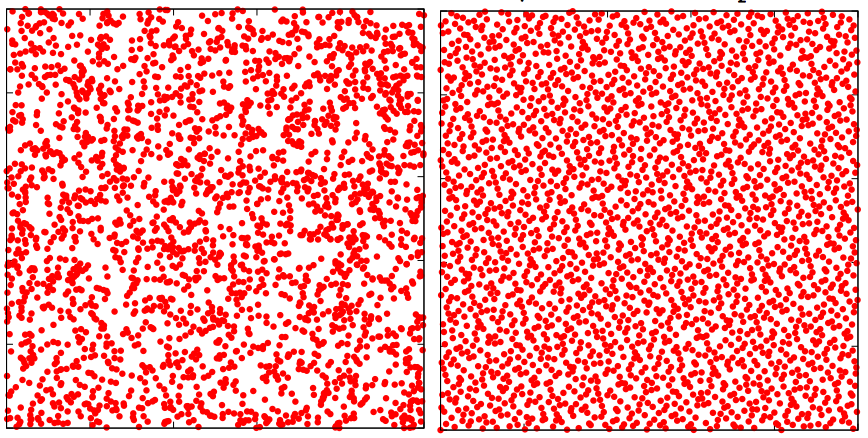
In order to avoid sampling artifacts (aliasing), DIRSIG4 uses unstructured sampling approaches in a variety of numerical integrals of spatial and angular domains. However, standard pseudo-random number generators have poor uniformity (and randomness) characteristics under normal operating conditions (see the example below). The effectiveness of adaptive sampling is dependent on getting very good coverage of the sampled domain. Additionally, since we don’t know ahead of time how many samples we’ll end up using, we need to make sure that we get that uniform coverage no matter how many samples we get. Therefore, instead of using a pseudo-random number generator, adaptive sampling uses a sampler from a class of "quasi-random" number generators with guaranteed uniformity. [1] Specifically, we use the Halton sequence, which appears random (though it is actually quite deterministic in generation) and has very good uniformity regardless of when you start/stop pulling samples. The example below shows what 2,500 samples look like when they are purely random (left) and quasi-random via the Halton sequence (right). Note the clusters and holes in the pure random pattern vs. the uniformity in the quasi-random pattern.
Hemispherical Sampling
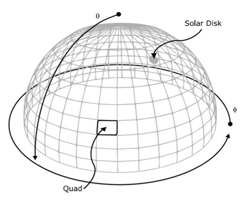
Most of the surface radiometry solvers in DIRSIG4 will sample the hemisphere above the surface in order to find the incident flux and weight it by the directional reflectance for that location within the hemisphere. In order to efficiently sample the hemisphere, most of the surface radiometry solvers partition the hemispherical into grid where each point in that grid is referred to as a "quad". Depending on the algorithm employed by a specific radiometry solver, it might sample each quad once, many times or not at all. Some solvers will attempt to figure out the most important quads to sample while others will use a brute force approach and sample all the quads. Typically the radiometry solvers have some sort of user-accessible control over zenith and azimuth resolution of the hemisphere grid, which can impact the performance of the algorithm.
Importance Sampling
When a surface is assigned a complex BRDF that has a significant contribution lobes (forward scattering, backward (retro) reflections, etc.), then it is desirable to concentrate on computing the contributions from the portions of the hemisphere where the magnitude of the BRDF is high rather than spend computation time where it is low. In order to facilitate this, some of the radiometry solvers use importance sampling (driven by the BRDF or BTDF) to sample the hemisphere above (or below) the surface.
User Configured Radiometry Solvers
The following section describes the "primary" radiometry solvers that the user configures for each material.
Classic Radiometry Solver [Surface]
The original DIRSIG radiometry solution for a surface was originally split into two classes of surfaces: either purely diffuse or purely specular. Late in the DIRSIG2 generation of the model (early 1990s), the calculations were modified so that a surface could modeled as a linear combination of specular and diffuse calculations.
The Classic radiometry solver was the first solver to be implemented within the DIRSIG4 radiometry framework. This solver was specifically written to reproduce the radiometry calculations implemented in the DIRSIG3 generation model, which had only a single surface leaving radiance calculation vs. the modular radiometry solver architecture in DIRSIG4.
|
|
The term "classic" is used within DIRSIG4 to denote any feature that was specifically implemented to reproduce calculations from the DIRSIG3 generation model. |
As the development of DIRSIG4 evolved, the "classic" radiometry solver was joined by alternate solvers with more robust numerical radiometry approaches.
Assumptions
The Classic radiometry solver in DIRSIG4 is based on this "diffuse
plus specular" type of solution. Furthermore, this solver only works
with materials assigned the
Classic Emissivity optical
property model (an error will be issued at init() time if this is
not the case). This latter requirement is because the solver directly
leverages the "specularity" parameter of the
Classic Emissivity
model to drive the "diffuse plus specular" partitioning.
|
|
The DIRSIG2 and DIRSIG3 models did not have a modular library of different optical properties. When the reflectance calculations were added to DIRSIG2, the reflectance (r) was computed as the emissivity (e) minus 1 (r = e - 1). The "specularity" term was then introduced as a spectrally constant scalar partitioning of how much of the reflectance was purely specular and how much was purely diffuse. |
Approach
The algorithm for the Classic radiometry solver is as follows:
-
A single ray samples the sun (if it is above the surface)
-
A single ray samples the moon (if it is above the surface)
-
A single ray samples the specular direction (if the emissivity model has a specularity of greater than
0). -
The diffuse irradiance term is incorporated as either:
-
The integrated sky irradiance (no hemispheric sampling), or
-
The hemispherically sampled sky irradiance
-
These resulting irradiance terms are then incorporated into specular and diffuse reflected radiance components. The "specular" reflected radiance is:
\begin{equation*} L_\mathrm{spec} = \frac{1 - \epsilon(\theta)}{\pi} ( E_\mathrm{sun} + E_\mathrm{moon} + E_\mathrm{spec} ) \end{equation*}
Note that the emissivity file might contain
spectrally-constant angular fall-off coefficients which make the
emissivity a function of declination (theta) angle. Because of the
spectrally-constant nature of these fall-off coefficients (the
EMS file only supports scalar coefficients), most
emissivity files have constant angular coefficients of 1.0 these
days.
The "diffuse" reflected radiance is:
\begin{equation*} L_\mathrm{diff} = \frac{1 - \epsilon(0)}{\pi} ( E_\mathrm{sun} + E_\mathrm{moon} + E_\mathrm{diff} ) \end{equation*}
Note that if the incident diffuse irradiance is hemispherically sampled, it is done so on a rigid 15 degree zenith and 30 degree azimuth grid. Also, the emissivity used to compute the reflectance for the diffuse component always uses the nadir (theta = 0) fall-off coefficient rather than using the appropriate fall-off coefficient for each angular sample.
The final reflected radiance is then the spectrally constant, weighted combination of the two terms:
\begin{equation*} L_\mathrm{total} = (S) \cdot ( L_\mathrm{spec} ) + (1-S) \cdot ( L_\mathrm{diff} ) \end{equation*}
where S is the spectrally constant "specularity" term supplied by the Classic Emissivity optical property model.
|
|
Both the specular and diffuse radiance components include the full sun and moon irradiance rather than these source terms being partitioned between them. That means that shadows appear in purely specular surfaces even if the sun (or moon) is not in the specular direction. |
Parameters
The user can enable diffuse hemisphere sampling via the
ENABLE_SAMPLED_DIFFUSE variable.
Strengths
There are no strengths of this radiometry solver compared to the more robust solvers available in DIRSIG4. This solver was implemented entirely to provide backward compatibility with DIRSIG3 and scene databases developed during the DIRSIG3 era.
Limitations
The following limitations should be considered when using the Classic radiometry solver:
-
The "specular + diffuse" model is driven by a spectrally constant parameter (see the "specularity" variable in the "Classic Emissivity" optical property model).
-
The source (sun and moon) irradiance is included in both the specular and diffuse components, rather than being partitioned between them. As a result, you see sun/moon shadows in 100% specular materials (which you should not) and you will not see sun/moon glints in 100% specular materials.
Generic Radiometry Solver [Surface]
The goal of the "Generic" radiometry solver is to effectively sample an unknown bi-directional reflectance distribution function (BRDF) in order to integrate the reflected radiance into a given direction. The current version of this radiometry solver is a redesign of an earlier solver that used a rigid, uniform grid sampling of the BRDF for the non-solar contributions. There were a few problems with this approach:
-
Regular sampling of any space can lead to aliasing artifacts
-
This was mitigated to some extent in two dimensions by rotating the sample "disks" within the sampling dome
-
-
Many (computationally expensive) samples could be wasted when the corresponding reflectance was relatively low
-
When the number of samples we wanted to take was few in number, it was very easy to miss high reflectance samples
-
There was no knowledge of the non-primary illumination sources which could be used to further direct the samples
The motivation for the redesign was the challenge to define a unified approach that addressed these problems. The "generic" radiometry solver encompasses an attempted solution to items 1-3, but a general, integrated solution to item 4 does not yet exist in this format.
|
|
There are a number of techniques that use forward Monte Carlo propagation of "importons" (nodes that point back to important sampling directions) that could be used to address the illumination problem. The importons are stored in a structure such as a k-nearest neighbor map or facet caches and can be searched to find the important sample directions. |
This is the most flexible of the surface oriented radiometry solvers. It employs importance sampling of the BRDF. It supports generation dependent fidelity. It is the universal powertool in that it can solve almost any problem really well. However, it isn’t optimized for any particular problem either. So some problems can take a very long time to solve. It has a large number of complex parameters that the user needs to be familiar with.
Assumptions
Assumptions were made about the BRDF in order to design this class:
-
The BRDF is not purely specular or purely diffuse
-
These types of BRDFs can be importance sampled directly and integrated using a Monte-Carlo approach
-
-
The BRDF cannot be analytically inverted
-
Again, a simple Monte-Carlo approach would be more effective
-
-
The BRDF is made up of some arbitrary combination of diffuse, specular, retro-reflective, and/or other components
-
For example, models or measurements where uniform sampling of the BRDF would not be efficient or effective
-
Approach
A threefold approach to sampling was taken in resolve the limitations discussed previously. The three sampling components are listed below.
-
The primary (solar) illumination vector is always sampled if it is on the same side of the geometry as the exitant vector
-
An abstract representation of the entire BRDF is used to importance sample non-primary contributions (the user determines the number of these importance samples per generation via the interface)
-
The un-sampled portions of the hemisphere integral are "cheaply" sampled to make sure that we don’t miss important source contributions
These three components ensure a thorough sampling of the surrounding space while attempting to make sure that each computationally expensive sample is as effective as possible. The parameters that are exposed to the user enable higher quality calculations at the expense of computational efficiency (or vice versa). Each component is now covered in detail.
Primary Illumination Samples
Under normal circumstances, the potential contribution from the sun is the most important in the BRDF integral, often orders of magnitude greater than other contributions. Since it is quite possible for the surface being calculated to be facing away from the sun, we make sure to check whether the solar vector is in the hemisphere defined by the surface normal. The solid angle of the sun is calculated once (static) by placing a virtual solar disk at distance one (to make calculations easy) corresponding to the solar half angle provided by the atmosphere model.
The appropriate geometry is calculated for the sample, but before any ray tracing begins, we make sure that the reflectance for that vector pair is significant (currently greater than 1e-6). The radiance from the solar vector is calculated via the usual DIRSIG problem/solution routines and the contribution is computed by applying the (already calculated) reflectance and solid angle.
Finally, we set the quad (see below) corresponding to the sun vector to the solar value calculated. If the solar solid angle is smaller than the quad solid angle then we calculate an approximate contribution from the remaining portion of the quad and add it to the stored value. If not, then we "squish" the entire contribution into one quad. This approach works since we make sure later that none of the sample vectors fall within the solar solid angle.
BRDF Importance Samples
The hemisphere corresponding to the contributions to the BRDF is modeled conceptually as a dome divided into quads that represent equal solid angles. This setup enables us to use the same solid angle for each quad calculations and effectively gives each sample region the same weight.
At this point, we do not sample each quad in the hemisphere to calculate the contribution to the reflected radiance. Instead, we choose important samples from a pre-computed importance mapping of the BRDF using a "factored sampler" (see the Appendix). This code will first choose a quad based on its relative weighting and then sample uniformly within the quad to arrive at the final sample. Using this method, it is quite possible to get many samples in a few quads and no samples in others. This is intentional. The idea here is that in important regions of the BRDF (as determined by the importance sampling) more samples are needed in order to calculate the average radiance from the quad. In other words, a mistake in a highly reflective quad is much more important than a mistake in a low reflectance quad, so we sample accordingly.
The total number of samples used in this component of the model is determined by the user (see the interface that follows). Additionally, the user defines the number of quads to use in terms of the number of zenith and azimuth samples. Given the sampling method, the effect of changing the number of quads is not particularly evident except for extreme values.
Cheap Source Samples
As stated in the previous section, it is possible for a quad to not get any samples and, therefore, not contribute to the hemispherical integral. The final component of this model is to do a "cheap" (computationally inexpensive) evaluation of whether there is a direct contribution to those quads (i.e. radiance incident from an official source or a emissive object). This is done by setting the generation of the sample to some arbitrarily high number. If the sample hits a source (e.g. the atmosphere) then the source radiance is returned.
Basic Parameters
The table and descriptions below outline the various parameters associated with this radiometry solver.
| Parameters | Default |
|---|---|
|
100 |
|
3 |
|
2 |
|
10 |
|
20 |
|
1 |
The following descriptions summarize the function of each variable:
INITIAL_SAMPLE_COUNT-
This variable defines the importance sample count used in the first bounce generation (the direct view). These samples are distributed in the hemisphere based on the magnitude of the BRDF.
SAMPLE_DECAY_RATE-
This variable controls how many importance samples are used after the first generation. The number of importance samples for a given bounce generation (i) is computed as Ni = N0/ratei, where N0 is the
INITIAL_SAMPLE_COUNTand rate is theSAMPLE_DECAY_RATE. Recall that the generation starts at0for the surface directly viewed by a detector. Hence using the default N0 = 100 and the default decay rate = 2, we can compute the number of samples for each generation as N1 = 100/21 = 50, N2 = 100/22 = 25, N3 = 100/23 = 12, etc. MAX_BOUNCES-
This variable controls after which bounce generation the reflected contribution is no longer computed. After this bounce generation is reached, only the thermal emission is computed.
MU_SAMPLESandPHI_SAMPLES-
These variables define the number of cosine distributed zenith angles and azimuthal angles, respectively, in the quad representation. The product of these two variables is the total number of quads in the sampling hemisphere.
SUN_SAMPLES-
This variable controls the number of samples used to sample the Sun disk.
|
|
The default parameters are set to conservative values that can capture the details of a complex BRDF. As a result, the solver will perform a very rigorous calculation that will take a long time. The user will probably want to change the parameters for a simpler surface. |
|
|
An INITIAL_SAMPLE_COUNT that is greater than or equal to the
total number of quads does not guarantee that every quad gets
an initial sample. That is because the BRDF might be highly
specular, which would place more samples in the specular region
of the hemisphere rather than distribute these samples uniformly.
|
Advanced Parameters
The hemispherical sampling and fidelity of the solutions used in the sampling of that hemisphere can be accessed by a set of advanced parameters that are not available in the graphical Material Database Editor.
|
|
These advanced parameters can have a massive impact on the accuracy and performance of the solver. These parameters should only be manipulated by an advanced user that is very familiar with the solver and how to correctly use these parameters. |
| Parameters | Default |
|---|---|
|
1 |
|
TRUE |
|
FALSE |
The following descriptions summarize the function of each advanced variable:
MIN_QUAD_SAMPLES-
When the surface sampler generates less than this minimum number of samples for each quad, quick samples are generated until the minimum is met.
PERMIT_DIRECT_ONLY-
The algorithm outlined before states that after the quads containing primary sources (Sun and Moon) are sampled, a limited set of importance samples are generated that sample additional quads. At this point there are still quads without enough samples, which are filled with cheap/quick samples. Setting the
PERMIT_DIRECT_ONLYflag toFALSEforces all these cheap/quick samples to be full samples. This flag is useful when the user wants to force high fidelity calculations to be used for all quads. TARGETS_ONLY-
When the solver constructs the set of samples, it beings with samples for specific source objects (Sun, Moon) and different directions (specular reflection, Snell transmission). This creates an initial set of "target quads" that are getting samples. The remaining quads are sometimes called "background quads", which are then sampled using other methods. If the
TARGETS_ONLYflag is set toTRUE, then the list of sampled quads only includes the "target quads" and the "background quads" are skipped. This can be useful for (a) materials that are very specular and/or (b) materials that are illuminated by a very directional sky (for example, UniformAtm with the Sky Fraction set to0).
| Parameters | Default |
|---|---|
|
8 |
|
2 |
|
100 |
The following descriptions summarize the function of each variable:
J_RANK,K_RANKandITERATIONS-
These parameters are used by the "factored sampler" to compress the BRDF into a form that can be used to importance sample the incident illumination directions given the exitant (view) direction.
Suggestions
The following are some suggestions and guidelines.
-
The
INITIAL_SAMPLE_COUNTandSAMPLE_DECAY_RATEdefine the number of importance samples used in each bounce generation. -
The
MAX_BOUNCESlimits the number of generations that full reflective calculations are performed on. After this maximum generation has been reached, the solver returns 0 radiance. -
Increasing the number of initial importance samples will better resolve the contributions from a complex (multi-lobe) BRDF.
-
Increasing the hemisphere grid resolution without increasing the number of importance samples will increase the accuracy of a problem like a graybody cavity, where multiple bounce thermal emission dominates.
-
Increasing the number of
SUN_SAMPLESwill resolve the penumbra, etc. (NEED MORE, include Gartley’s example?). -
If the hemispherical reflectance (angularly weighted average of the BRDF) is low and/or the BRDF is very diffuse, then a larger decay rate might be employed since the radiance reflected by any given sample will contribute little to the overall result.
Strengths
The following are "strengths" of the Generic radiometry solver:
-
Because it incorporates importance sampling driven by the BRDF (via the "factored sampler") it can be very good at reproducing a complex (multi-lobed) BRDF.
Limitations
The following limitations should be considered when using the Generic radiometry solver:
-
The interfaces to the solver are complex. It is easy to "dial up" the fidelity of the solver to get robust results, but the computation times might be long. Tuning the solver to provide robust results in reasonable times can be harder.
-
Ideally this solver would have a "numeric convergence" mechanism rather than simply a "number of samples" mechanism. Being able to tell the solver that you would like the leaving radiance to converge (controlled by some sort of fitness parameter) might be preferable.
Simple Radiometry Solver [Surface]
The Simple radiometry solver (SRS) was introduced in 2013 as a compromise between the power and complexity of GRS and the simplicity and speed of CRS. As long as a few basic assumptions are met, the Simple rad solver can meet or exceed the radiometric fidelity of GRS while offering performance closer to CRS.
Assumptions
The following key assumptions influenced the design of the algorithm.
-
The BRDF can be adequately described by a diffuse + specular lobe model
-
The specular lobe (if there is one) is found automatically
-
No restrictions are placed on the width of the lobe
-
The specular lobe is assumed to have its peak more or less in the specular direction
-
The specular lobe is assumed to be rotationally symmetric
-
-
Primary illumination is driven by the sun, the moon and whatever is in the specular direction.
-
Secondary illumination is currently driven by a sky and not by diffuse illumination by background objects.
-
This limitation may be removed in the future
-
-
Specular lobe contributors (i.e. surfaces subtended by the lobe solid angle) are assumed to be geometrically similar within a single class of material.
-
Except for some very extreme cases, this is a safe assumption to make
-
|
|
The Simple radiometry solver should only be used for objects diffusely illuminated by the Sky. It is not a good choice for indoor or exo-atmospheric objects since contributions from the diffuse portion of the BRDF will be poorly represented. |
Approach
The primary driver of this solver is a good estimate of the specular lobe (magnitude and shape) and the diffuse reflectance. At initialization time a model of the specular component is characterized with a symmetric falloff function for each sampled view angle. For each sampled view angle, the directional hemispherical reflectance (DHR) is then computed and split between the specular lobe and the remaining hemisphere. This specular and diffuse model is stored as a function of sampled zenith (declination) view angle, and the number of angles varies depending on a primary fidelity parameter (discussed later).
When the solver is called at compute() time, the following approach is
used to sample the incident illumination field:
-
One ray samples the sun and if the sun is not visible, one ray samples the moon.
-
Some care is taken to account for potential overlap of these samples (for example, the sun is in the specular direction).
-
-
Many rays are used to sample the specular lobe geometrically to find the materials (and proportions) subtended by the lobe solid angle
-
The radiometric contribution of the lobe is estimated from a unique, representative radiance from each material found, and weighted by the proportion of the lobe
-
-
The remaining hemisphere is sampled geometrically to determine the amount of sky light that reaches the surface
-
This is accomplished by a "shadowing" algorithm that randomly samples the hemisphere looking for objects that "shadow" or obscure portions of the sky. If an object blocks a portion of the sky then some portion of the total sky illumination is removed.
-
The shadowing algorithm takes into account the orientation of the surface (i.e. if the normal is horizontal it automatically shadows half the hemisphere).
-
|
|
The diffuse shadowing is based on geometry, not on material, so a mostly transmissive surface will still be considered to occlude the sky |
Parameters
The Simple radiometry solver has a very basic user interface. There are three levels of "quality" that determine how many samples are used for both the integrals, the resulting models and the number of shadow samples.
    RAD_SOLVER_NAME = Simple
    RAD_SOLVER {
        QUALITY = Medium
    }
| Internal Parameter | Low | Mediun | High |
|---|---|---|---|
Specular Lobe Model Angles |
30 |
30 |
90 |
Sky Shadow Samples |
10 |
100 |
200 |
Specular Samples |
200 |
200 |
1800 |
The specular lobe model angles are used to drive the fidelity of the pre-computed model. When a ray strikes a surface, computations are based on linearly interpolating the two closest values in the model to the view angle relative to the surface normal. The model data is stored at different degree intervals based on the quality. The values being stored per view angle are:
-
Specular lobe thresholds
-
This is the cosine of the angle corresponding to the maximum extent of the specular lobe measured relative to the specular direction. It is used to determine when to use the specular lobe or diffuse portions of the model.
-
The cutoff is based on the (spectral) maximum of the BRDF
-
-
Specular lobe solid angles
-
Specular lobe reflectance
-
This is the BRDF integrated over the specular lobe
-
-
Diffuse reflectances
-
This is the BRDF integrated over the portion of the BRDF not in the specular lobe
-
Because the interplay between the specular and diffuse portions of the BRDF is highly susceptible to small differences in integration, we calculate and maintain our values (rather than attempt to derive one from the other using an externally calculated DHR)
-
-
Specular falloff coefficients
-
This is a vector of values describing the value of the BRDF within the lobe at the cosine of the angle relative to the specular vector
-
This data is stored at a high sampling rate (10x the number of angles given by the quality) to better model the shape of the lobe
-
The value stored is based on the average value sampled at a constant angle around the specular vector (no user control over this sampling rate)
-
All spectrally varying values (reflectances and falloff) are stored spectrally.
Strengths
The following are "strengths" associated with the Simple radiometry solver:
-
Since there are not a large number of exotic material BRDFs available (i.e ones with retro-reflection or highly shaped diffuse portions of the BRDF), the reality is that most scenes will employ reflectance models that are close to a diffuse plus specular assumption
-
Although the sampling approach employed by this solver is much simpler than that in the Generic radiometry solver, it is well suited for these simple reflectance representations.
-
-
SRS runs much faster (usually one or more orders of magnitude faster) than GRS to produce the same absolute radiometry under the given assumptions.
-
SRS is less susceptible to noise than GRS since its sampling is very limited
Limitations
The following limitations should be considered when using the Simple radiometry solver:
-
It doesn’t incorporate light reflected by adjacent objects that fall within the diffuse portion of the BRDF.
-
Any given diffuse sample is either "sky" or "not sky".
-
-
This solver should not be used for indoor or exo-atmospheric objects.
-
Directions within the specular lobe are treated uniformly for background radiance (not sun/moon radiance) even though the lobe most likely not uniform.
-
It doesn’t handle BTDFs at the moment (but the Generic radiometry solver does).
-
It will not importance sample a complex BRDF (but the Generic radiometry solver does).
-
Off-specular lobes are currently re-aligned to the ideal specular direction and will have a slightly wider width than they should.
Mirror Radiometry Solver [Surface]
The Mirror radiometry solver exists to address the need to quickly configure a material that is a "perfect reflector":
-
The surface is reflects whatever is in the specular direction.
-
There is no "color" to the surface (light is reflected equally at all wavelengths).
Assumptions
The Mirror radiometry solver is used to model "perfect reflector" or "mirror" surfaces only.
Approach
The Mirror radiometry solver handles specular reflections only, by only considering contributions from the specular direction.
Parameters
The Mirror radiometry solver has no options.
    RAD_SOLVER_NAME = Mirror
    RAD_SOLVER {
    }
Limitations
The Mirror radiometry solver can only be used to model perfect reflectors.
Null Radiometry Solver [Surface]
The "Null" radiometry solver exists to address a limited set of scenarios where a material does not need to have a surface leaving radiance calculation:
-
Proxy materials that are remapped via a material map.
-
Materials that are driven by a radiance map.
Assumptions
The "Null" radiometry solver does not perform any calculations.
Approach
The "Null" radiometry solver does not perform any calculations.
Parameters
The "Null" radiometry solver has no options.
    RAD_SOLVER_NAME = Null
    RAD_SOLVER {
    }
Limitations
The "Null" radiometry solver does not perform any calculations.
Automatically Configured Radiometry Solvers
The following is a description of the various radiometry solvers that are automatically configured by DIRSIG for each material. Because these solvers are automatically setup by the model, there are no user-defined parameters to configure.
Atmosphere Radiometry Solver
This solver forms the interface between the radiometry engine and the various atmospheric radiative transfer models that can be used with DIRSIG. This solver is in charge of returning important atmospheric radiometric components including path transmissions, path radiances, sky radiances, etc.
Boundary Radiometry Solver
This radiometry solver is used at the boundary between two built-in mediums. The most common example is the boundary between the atmosphere and space. This solver is in charge of making sure the current medium is correctly updated and that any "boundary" related effects are accounted for.
Transmission Radiometry Solver
This solver is in charge of computing the transmission through a given surface or volume. It is automatically setup when the user provides a material description that includes any transmissive aspects. Note that some radiometry solvers handle transmission directly, and this solver does not need to be used. For example, the Generic Radiometry Solver handles the transmitted radiation by performing a sampling of the bi-directional transmission function (BDTF).
Thermal Emission Radiometry Solver
This solver is in charge of computing the thermal emission of a surface or volume. It uses the temperature determined by the Temperature Solver, the Planck blackbody equation and the material optical properties (to determine the spectral emissivity).
Lidar Direct Radiometry Solver
This solver is in charge of computing the directly reflected laser energy for a simulation containing an active laser system.
Preview Radiometry Solver
This solver is used to replace any full solution radiometry solver during a Preview Mode simulation. This solver simply captures the material ID of the surface intersected rather than performing any rigorous radiometric calculation.
Secondary Sources Radiometry Solver
This solver is in charge of computing the reflected radiance from secondary (user-defined) sources.