Surface Optical Properties

This document describes the optical properties that can be associated with surface materials (hemispherical reflectances, bi-directional reflectance distribution functions (BRDFs), etc.) in a DIRSIG Material Database file.

Overview

Each surface optical property model has different features, strengths and weaknesses. To help users understand these at a glance, the following table is provided:

Table 1. List of surface optical property models
Name	Type	Distribution	Spectral	Spatial	Polarized*
Classic Emissivity	Emissivity	Diffuse	Varying	Varying	No
Delta Reflectance	Reflectance	Delta	Varying	Constant	No
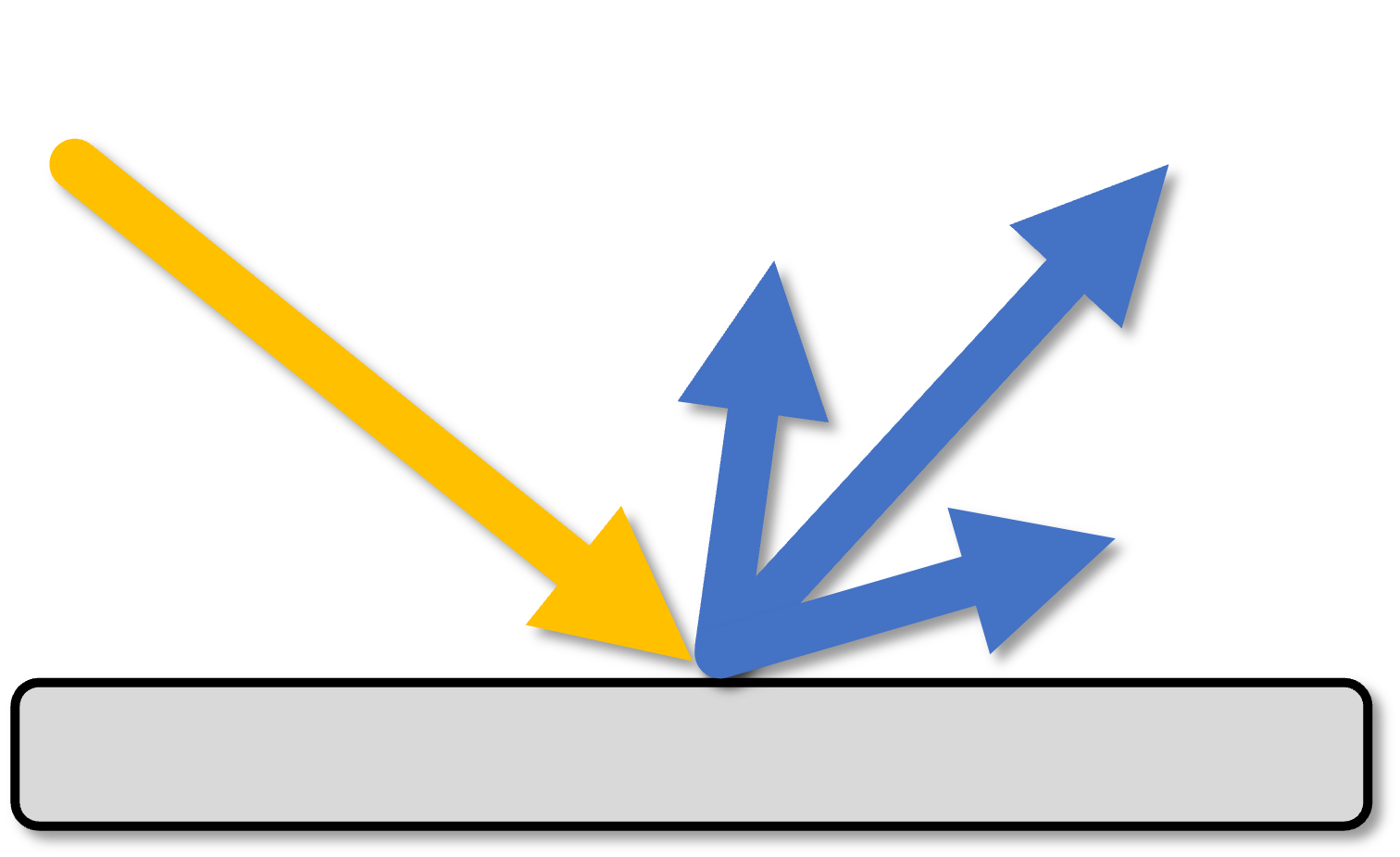
Priest-Germer BRDF	Reflectance	Bi-Directional	Varying	Constant	Yes
Ross-Li BRDF	Reflectance	Bi-Directional	Varying	Constant	No
Shell Background BRDF	Reflectance	Bi-Directional	Varying	Varying	Yes
Shell Target BRDF	Reflectance	Bi-Directional	Varying	Varying	Yes
Simple Reflectance	Reflectance	Diffuse	Varying	Constant	No
Spherical Data BRDF	Reflectance	Bi-Directional	Varying	Constant	No
Ward BRDF	Reflectance	Bi-Directional	Constant	Constant	No
RGB Map	Reflectance	Diffuse	Varying	Varying	No
Reflectance Map	Reflectance	Diffuse	Varying	Varying	No
Curve Map	Reflectance	Diffuse	Varying	Varying	No
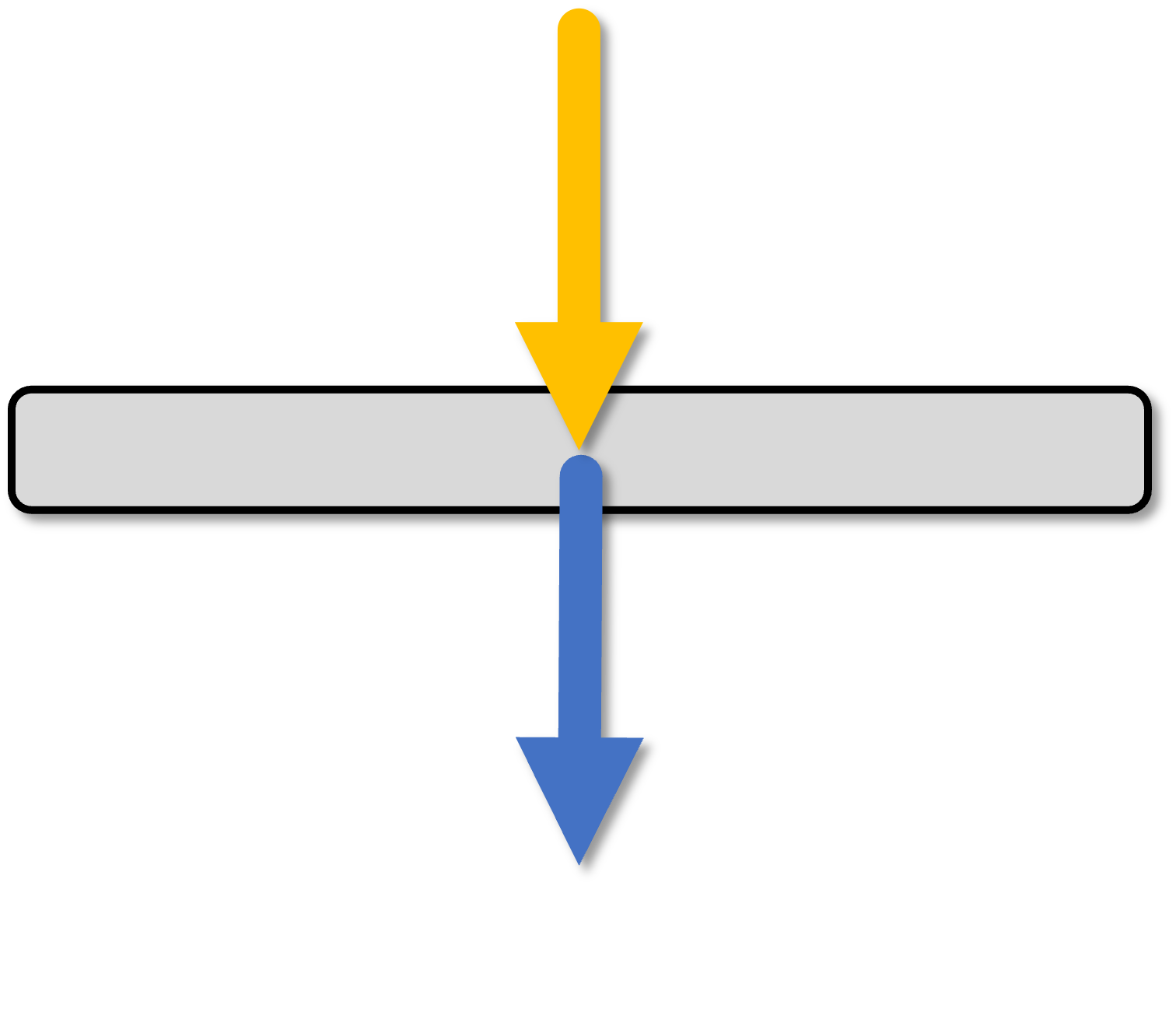
Delta Transmittance	Transmittance	Delta	Varying	Constant	No
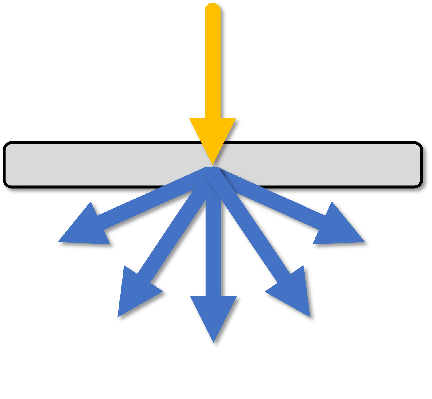
Simple Transmittance	Transmittance	Diffuse	Varying	Constant	No
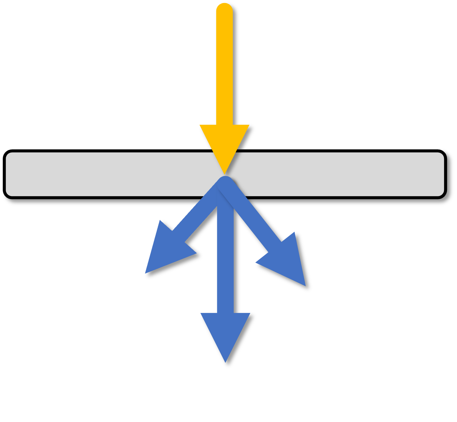
Spherical Data BTDF	Transmittance	Bi-Directional	Varying	Constant	No
Classic Extinction	Extinction	Diffuse	Varying	Constant	No

Polarization is only supported in DIRSIG4.

The attributes of each model are as follow:

Type: Is this property an emissivity, reflectance or transmittance model?
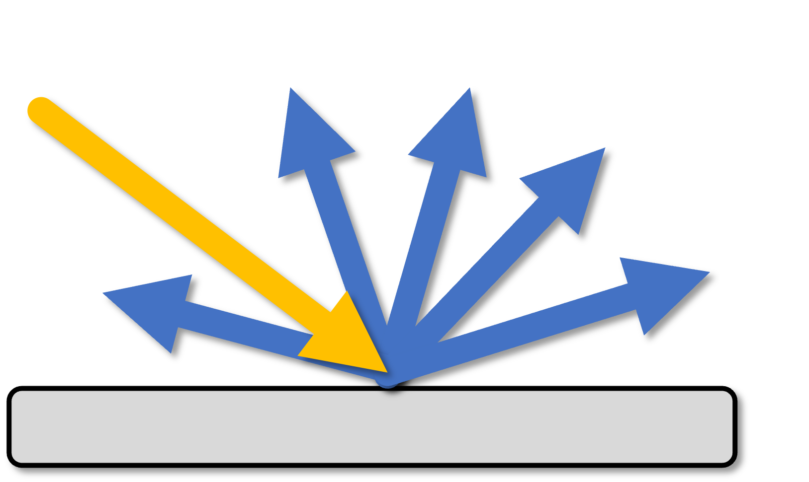
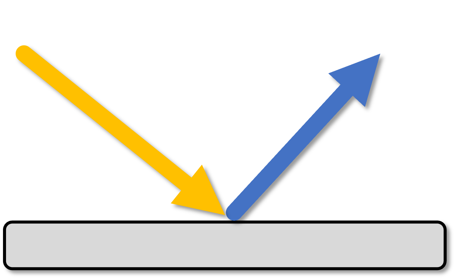
Distribution: Is the scattering distribution generally delta, diffuse (Lambertian), directional or bi-directional?
Spectral: Does the model (as currently implemented) provide a spectrally constant or spectrally varying results?
Texture: Does the model (as currently implemented) provide a mechanism to introduce spatial variability or what most users would call "texture"?
Polarized: Is the model capable of producing polarized results? (NOTE: Polarization is only available in DIRSIG4)

Inside DIRSIG4 the SurfaceProperties object provides an abstracted interface to the surface optical properties defined for a material. A calling object (for example, a radiometry solver) can ask for the emissivity and that quantity will be automatically computed if only a reflectance model is defined. Similarly, this object will also provide a reflectance if only an emissivity model is defined. The SurfaceProperties object can also hemispherically integrate a bi-directional reflectance distribution function (BRDF) to provide the appropriate directional hemispherical reflectance (DHR).

Materials are assumed to be in thermodynamic equilibrium which allows DIRSIG to apply Kirchoff’s rule to derive optical properties that may be missing from the definition (e.g. the spectral reflectance can be obtained from the spectral emissivity by assuming an R = 1 - E relationship). This conservation of energy based derivation can only be applied to the "total" property (e.g. the directional hemispherical reflectance), but nothing can be directly derived about the distribution (e.g. the bi-directional reflectance distribution function).

Emissivity Properties

Emissivity properties are supplied via the EMISSIVITY_PROP in the SURFACE_PROPERTIES of the material file.

Classic Emissivity

The ClassicEmissivity model was implemented in DIRSIG4 as a method to provide backwards compatibility (in terms of both input file format and mathematical behavior) to the spectral emissivity support in DIRSIG2 and DIRSIG3. Although this property is defined by spectral emissivity data, it is widely used across the emissive and reflective regions in many DIRSIG scenes as the way to model diffuse reflectance with spatial variation.

Figure 1. Diffuse reflectance distribution.

Background

In addition to providing backward compatibility to earlier versions of the DIRSIG model, this optical property provides a bulk of the functionality for the texture map mechanism.

Setup and Options

The configuration for this optical property is composed of an external, spectral emissivity file (which may contain multiple spectral measurements) and a spectrally-constant parameter that attempted to capture

EMISSIVITY_PROP_NAME = ClassicEmissivity
EMISSIVITY_PROP {
    FILENAME = dirt.ems
    SPECULARITY = 0.0
}

See this section in the property maps manual to see how this property can be configured with a texture map.

Input File

The format of the spectral emissivity file provided via the FILENAME variable is described in detail in a separate document. The SPECULARITY variable is used by the Classic Radiometry Solver to partition the reflected radiance into diffuse and specular contributions. However, the fact that this parameter is spectral constant is considered a major limitation of this property. In most cases, this model is used with the SPECULARITY set to 0, which forces the model to have diffuse (Lambertian) characteristics.

A TEXTURE_MAP can be directly defined in this property. For more information see the example in the Maps Manual.

Examples

Most of the standard scenes distributed with the DIRSIG model contain multiple examples of the ClassicEmissivty model in use.

References

J.R. Schott, C.N. Salvaggio, S.D. Brown and R.A. Rose, "Incorporation of texture in multispectral synthetic image generation tools", Proc. of SPIE, Targets and Backgrounds: Characterization and Representation, Vol. 2469, No. 23, April 1995

Reflectance Properties

Reflectance properties are supplied via the REFLECTANCE_PROP in the SURFACE_PROPERTIES of the material file.

Delta Reflectance

The DeltaReflectance model is a bare bones reflectance optical property with a frontside distribution that is Delta (light is only forward scattered).

Figure 2. Delta reflectance distribution.

Background

This optical property was introduced in DIRSIG5 as a simple way to model highly directional reflectances.

Setup and Options

The DeltaReflectance model can be configured with an external, two column ASCII/Text file containing wavelength (in microns) and reflectance pairs via the TXT_FILENAME variable:

REFLECTANCE_PROP_NAME = DeltaReflectance
REFLECTANCE_PROP {
    TXT_FILENAME = glass.txt
}

This propoerty can also be configured with an external ENVI spectral library (SLI) file using the SLI_FILENAME and SLI_INDEX variables:

REFLECTANCE_PROP_NAME = DeltaReflectance
REFLECTANCE_PROP {
    SLI_FILENAME = glass.sli
    SLI_INDEX = 0
}

where the SLI_INDEX is the zero-based index for the curves in the SLI file. Alternatively you can use the SLI_SPECTRUM variable to select a curve using the name associated with it.

REFLECTANCE_PROP_NAME = DeltaReflectance
REFLECTANCE_PROP {
    SLI_FILENAME = glass.sli
    SLI_SPECTRUM = uncoated
}

Input File

The input file is currently assumed to be a two-column, space delimited (space or tab), ASCII/Text file containing wavelengths in microns and reflectances as a fraction. The spectral data is linearly interpolated to compute wavelengths between those provided. The simple example below shows a file that describes a 10% reflectances for the UV through the LWIR wavelengths.

 0.20 0.10
...
[lines deleted for documentation purposes]
...
20.00 0.10

Examples

References

None.

Priest-Germer BRDF

The Priest-Germer BRDF model is a polarized version of the Torrance-Sparrow BRDF model, where the polarized component is driven by the complex index of refraction.

Background

Like many of the theoretical (physical) BRDF models, this model computes the BRDF based on a mathematical formulation that is derived from theory. The major advantage of the formulation developed by Priest and Germer over the classic Torrance and Sparrow formulation was that polarized BRDF values could be computed for a broad range of materials that had existing Torrance-Sparrow BRDF parameters. However, in practice, the Torrance-Sparrow BRDF model parameters are usually fit to unpolarized, measured data. Without proper fitting constraints, some complex index of refraction values derived from the unpolarized measurements were not physically realistic. Although the Torrance-Sparrow BRDF calculation reproduced the measured data well, using the fitted parameters to predict polarized BRDFs with the Priest-Germer BRDF calculation can sometimes result in unrealistic polarization behavior.

The Priest-Germer model is still considered a decent BRDF model for surfaces that do not feature a lot of sub-surface scattering. Therefore, it is useful to describe bare metals. Although the overall reflectance of a painted metal surface might be correct, the lack of a sub-surface scattering model usually results in an over estimation of polarization (sub-surface scattering tends to depolarize incident energy).

Setup and Options

The model needs the slope variance and the complex index of refraction, as a function of wavelength. The following is an example excerpt from a DIRSIG material file showing the setup of this model:

REFLECTANCE_PROP_NAME = PriestGermer
REFLECTANCE_PROP {
    PARAMETER_FILE = aluminum.brdf
    ENABLE_POLARIZATION = TRUE
    ENABLE_DIFFUSE_CONTRIBUTION = TRUE
    ENABLE_SHADOWING_FUNCTION = TRUE
}

The options are defined as:

ENABLE_POLARIZATION: Enable the polarized BRDFs to be generated. When not enabled, the model returns 100% depolarizing BRDFs.
ENABLE_DIFFUSE_CONTRIBUTION: Enable the inclusion of a DHR-based diffuse contribution. Note that this feature was not included in the original description of the model.
ENABLE_SHADOWING_FUNCTION: Enable the the "shadowing function" described by Torrance-Sparrow. Note that this feature was not included in the original description of the model.

Input Parameter File

The input parameter file has four columns of data:

The wavelength in microns
The surface normal variation, or sigma (in radians)
The complex index of refraction, real part
The complex index of refraction, imaginary part

A sample parameter file in its entirety:

0.53904 0.150 0.826 6.283
0.56354 0.150 1.018 6.846
0.61990 0.150 1.304 7.479
0.66677 0.150 1.741 8.205
0.77487 0.150 2.625 8.597

Examples

Consult the following demos for materials using this model:

The Polarization1, Polarization4 and Polarization5 demos all use the same subject scene configuration that includes several materials assigned the Priest-Germer BRDF model.

References

J. P. Meyers, "Modeling Polarimetric Imaging using DIRSIG", Ph.D. Thesis, Center for Imaging Science , Rochester Institute and Technology, 2002 (link to PDF).
R. Cook and K. Torrance, "A reflectance model for computer graphics", Computer Graphics (SIGGRAPH '81 Proceedings), Vol. 15, No. 3, pp. 301-316, July 1981.
R.G. Priest and S.R. Meier, "Polarimetric microfacet scattering theory with applications to absorptive and reflective surfaces", Optical Engineering, Vol. 41, No. 5, pp 988-993, May 2002.
R. G. Priest and T. A. Germer, "Polarimetric BRDF in the Microfacet Model: Theory and Measurements", Proceedings of the 2000 Meeting of the Military Sensing Symposia Specialty Group on Passive Sensors, Vol. 1, 169-181, 2000.

Ross-Li BRDF

The Ross-Li BRDF model is an implementation of the kernel based BRDF described in Wanner et al. 1995 paper, where the Ross and Li in the name refers to the kernels developed by Ross (1981) and Li (1992). They are used in linear combination (along with a uniform, isotropic term) to form the final BRDF that varies with wavelength. Specifically, the reflectance is of the form

\( R = C_{\mbox{iso}} + C_{\mbox{geo}}K_{\mbox{geo}} + C_{\mbox{vol}}K_{\mbox{vol}}\)

where the vol (volume-scattering (radiative transfer) based) and geo (geometric optics based) kernels and coefficients refer to the Ross and Li kernels, respectively.

Background

The Ross-Li BRDF model is intended to capture the aggregate reflectance of vegetated land surfaces at very large scale (100m to kilometers). It has the advantage that it can be derived from satellite imagery by fitting measured data from many scans of the same area (e.g. Ross-Li fitted BRDFs are a product of MODIS).

There are two forms of each kernel implemented in the DIRSIG model. The Ross kernel has a thick (large leaf area index (LAI) values) version and a thin version (small LAI). The equations used for each form of the kernel are:

\begin{equation*} K_{\mbox{thick}} = \frac{\left(\pi/2 - \xi\right)\cos\xi + sin\xi}{\cos\theta_i + \cos\theta_v}-\frac{\pi}{4}, \end{equation*} \begin{equation*} K_{\mbox{thin}} = \frac{\left(\pi/2 - \xi\right)\cos\xi + sin\xi}{\cos\theta_i\cos\theta_v}-\frac{\pi}{2}, \end{equation*}

where the phase angle of scattering is defined as

\begin{equation*} \cos\xi = \cos\theta_i\cos\theta_v + \sin\theta_i\sin\theta_v\cos\phi , \end{equation*}

and the i and v subscripts to the zenith angles refer to incident and view directions, respectively, and the azimuth angle is measured between the two directions. For more details and the derivation, see the article referenced below.

The Li(-Strahler) model similarly has two forms, a sparse kernel (ignores mutual shadowing) and a dense version (incorporates mutual shadowing). The Li kernel takes two parameters that describe the crown shape and relative height (BR (b/r) and HB (h/b), where h is the height, b is the width and r is the minor axis length of an ellipse describing the crown. Rather than show the equations for each (see reference for the form), the below plot shows kernel values computed for each while varying the input parameters:

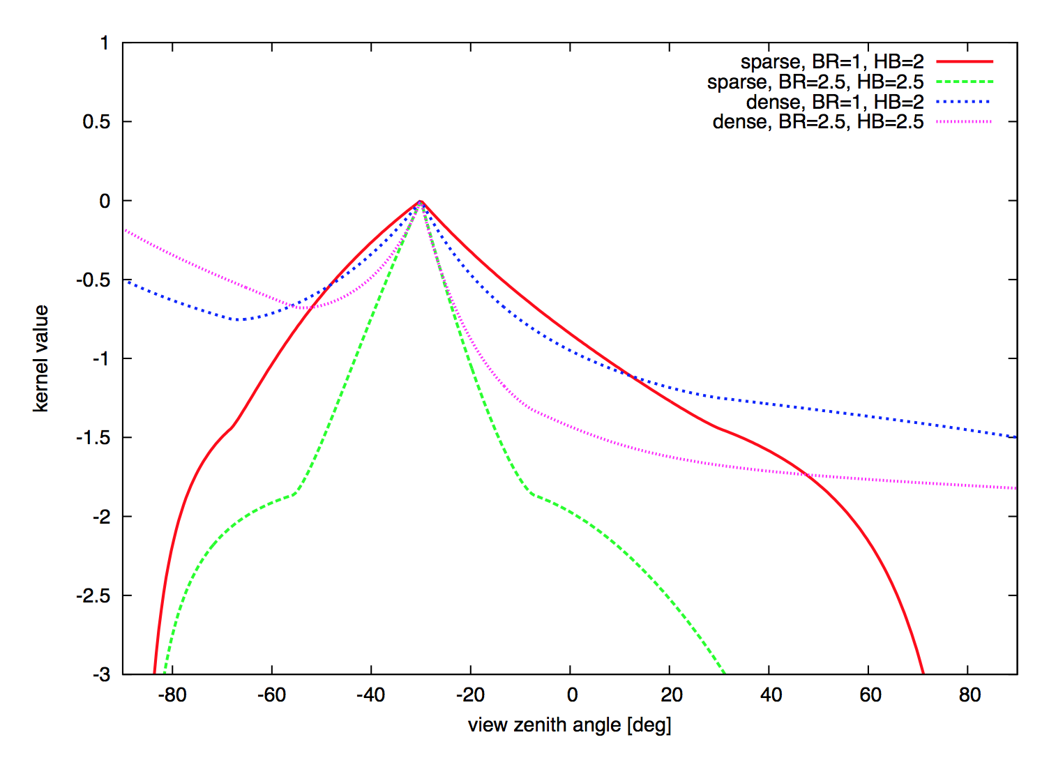
Note that the peak seen at -30 degrees is the characteristic "hotspot" of forest canopy BRDFs.

Setup and Options

The RossLi BRDF is setup by supplying the model to be used (choice of variant for each of the kernels) and the canopy descriptors if need. By default DIRSIG will assume a Ross-Thick and Li-Sparse model (as is used by MODIS) with a BR of 1 and HB of two. Then the user supplies the fit values for each desired wavelength (fit parameters are interpolated between supplied wavelengths and "flat" extrapolated beyond the minimum/maximum). Each set of fit parameters is supplied in its own entry.

REFLECTANCE_PROP_NAME = RossLi
REFLECTANCE_PROP {

    ROSS = THICK
    LI = SPARSE
    BR = 1.0
    HB = 2.0

    BRDF_FIT {
        LAMBDA = 0.645
        FISO   = 0.101
        FVOL   = 0.032
        FGEO   = 0.018
    }

    BRDF_FIT {
        LAMBDA = 0.858
        FISO   = 0.260
        FVOL   = 0.081
        FGEO   = 0.042
    }
}

Alternatively, a file can be read in which has the same data in column format, wavelength (Microns), FISO, FVOL, and FGEO, e.g.

0.645 0.101 0.032 0.018
0.858 0.260 0.081 0.042

and

REFLECTANCE_PROP_NAME = RossLi
REFLECTANCE_PROP {

    ROSS = THICK
    LI = SPARSE
    BR = 1.0
    HB = 2.0

    BRDF_FIT_FILE = file.fit
}

which is equivalent to the first version.

Examples

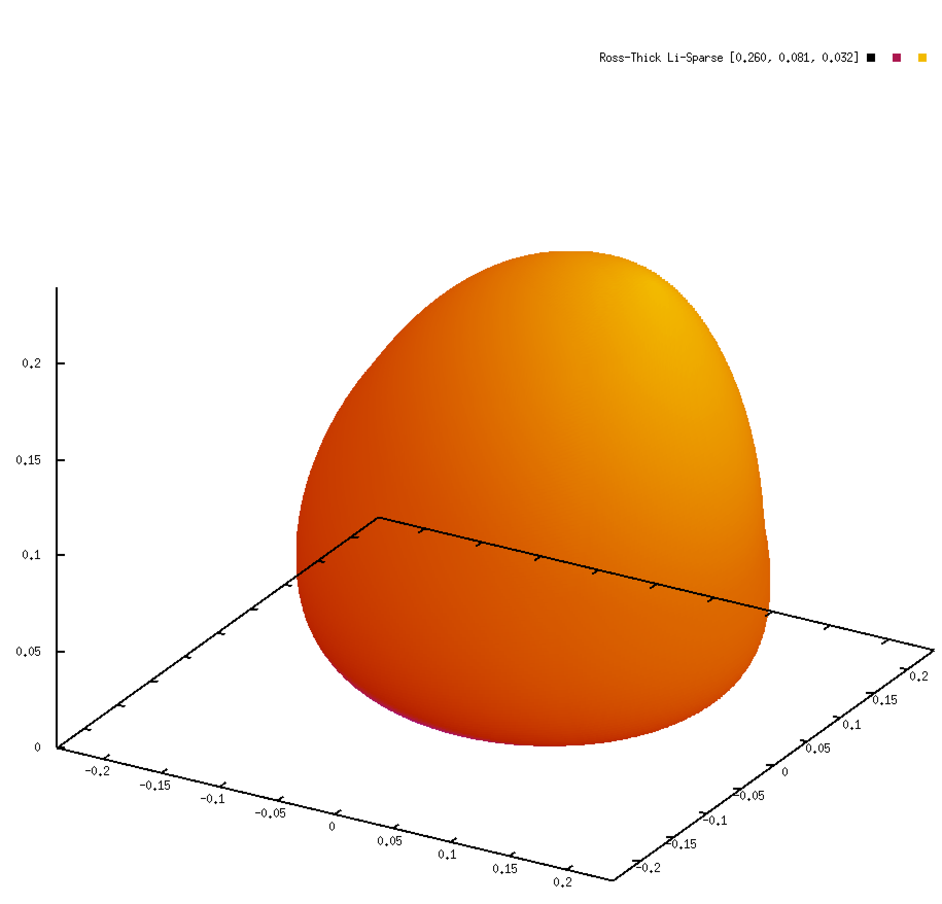
The following plot is of the BRDF produced for a 30 degrees source based on the inputs above, for 858 nanometers:

References

Wanner, W., X. Li, and A. H. Strahler (1995), On the derivation of kernels for kernel-driven models of bidirectional reflectance, J. Geophys. Res., 100(D10), 21077-21089.

Shell Target Reflectance

The ShellTarget BRDF model was developed by James Shell at RIT as a key component of his Ph.D. dissertation. The model can compute polarized reflectances for "target" (man-made) materials. A parameter file holds model fit data at measured wavelengths. A DIRSIG emissivity file is used to help interpolate and extrapolate for other wavelengths.

Background

The ShellTarget BRDF model employs many of the same terms created in other models for both the surface normal distribution (Cauchy), shadowing term (Maxwell-Beard) and volume scattering term (Maxwell-Beard);

The Cauchy distribution

\begin{equation*} p_C(\theta_N) = \frac{B}{cos(\theta_N)[\sigma^2 + tan^2(\theta_N)]} \end{equation*}

The Maxwell-Beard shadowing function

\begin{equation*} S_{MB} = \frac{1+\frac{\theta_N}{\Omega}e^{-1\beta/\tau}}{1+\frac{\theta_N}{\Omega}} \end{equation*}

The Maxwell-Beard volume term

\begin{equation*} V_{MB} = \rho_D + \frac{2 \rho_V}{cos(\theta_i) + cos(\theta_r)} \end{equation*}

Setup and Options

The material database entry simply specifies the fit and emissivity files:

REFLECTANCE_PROP_NAME = ShellTarget
REFLECTANCE_PROP {
    BRDF_FIT_FILE = black_paint.fit
    EMISSIVITY_FILE = black_paint.ems
    INTERPOLATION_METHOD = 1
}

The INTERPOLATION_METHOD parameter dictates how DIRSIG spectrally interpolates the ShellTarget BRDF based on the fact that the BRDF parameters are usually only specified at a handful of wavelengths (i.e 0.325, 0.6328, 1.06 etc..) while the spectral emissivity is specified at a much higher spectral resolution. Interpolation method 0 ignores the high spectral fidelity emissivity curve, and simply utilizes the BRDF parameter fit data and linearly interpolates between the reference wavelengths. Interpolation method 1 mimics the NEF database v10 handling of BRDF spectral interpolation, utilizing the higher spectral resolution emissivity curve to adjust the diffuse portion of the BRDF such that the hemispherically integrated BRDF model matches the measured diffuse hemispherical reflectance curve.

The job of spectrally interpolating a BRDF model leverages both pieces of information to hopefully bridge the gaps for accurate spectral, polarimetric image simulations and scene projections. We have encountered three different approaches to spectral interpolation which are summarized in the table below:

Table 2. Summary of BRDF Spectral Interpolation Approaches
Method	Description	Suitability	Requirements
`1`	Linear interpolation of modeled BRDF between reference wavelengths.	First surface dominated materials that have well known complex index of refraction values that adequately resolve all spectral features over desired wavelength range. Examples: Solid metals, optically opaque and homogeneous liquids.	Parameterized BRDF at a small number of sparsely spaced wavelengths.
`2`	Linear interpolation of 1^st surface scatter term of BRDF between reference wavelengths. Apply wavelength dependent gain to "bulk" scatter BRDF term such that the resulting hemispherical integration of full BRDF matches the lab measured DHR spectrum.	Materials possessing a combination of 1^st surface and bulk scattering behaviors for which the magnitude of the specular glint changes slowly in wavelength and the diffuse scatter changes quickly with wavelength Examples: car paints and some vegetation in the visible to near IR.	Parameterized BRDF at a small number of sparsely spaced wavelengths. High spectral resolution lab measurement of DHR. Resulting DHR of model equals lab measured DHR.
`3`	Linear interpolation of both 1^st surface and "bulk" scatter terms of BRDF between reference wavelengths with an additional wavelength dependent gain applied to model such that the resulting hemispherical integration of modeled BRDF matches the lab measured DHR spectrum.	Materials for which the 1^st surface scatter dominates, but is not the only contributor to the full BRDF magnitude and the complex index of refraction values are not known adequately. Examples: painted surfaces in the mid-wave and long-wave infrared.	Parameterized BRDF at a small number of sparsely spaced wavelengths. High spectral resolution lab measurement of DHR. Resulting DHR of model equals lab measured DHR.

The "fit" file contains the parameters for the BRDF model as a function of wavelength. An example .fit file follows:

SHELL_TARGET = 1.0

FIT_PARAMS {
    LAMBDA = 0.352
    N = 1.449
    K = 0.2146
    DHR = 0.0464

    ORIENT_PROB_NAME = Cauchy
    ORIENT_PROB {
        BIAS    = 0.0603
        SIGMA   = 0.3553
    }

    SHADOW_FUNCT_NAME = Maxwell-Beard
    SHADOW_FUNCT {
        TAU = 2.17
        OMEGA   = 1.47E+02
    }

    VOLUME_TERM_NAME = Maxwell-Beard
    VOLUME_TERM {
        RHO_D   = -1.06E-04
        RHO_V   = 5.29E-04
    }
}

FIT_PARAMS {
    LAMBDA  = 0.632
    N   = 1.405
    K   = 0.2289
    DHR = 0.0402

    ORIENT_PROB_NAME = Cauchy
    ORIENT_PROB {
        BIAS    = 0.0556
        SIGMA   = 0.3331
    }

    SHADOW_FUNCT_NAME = Maxwell-Beard
    SHADOW_FUNCT {
        TAU = 1.717
        OMEGA   = 1.19E+02
    }

    VOLUME_TERM_NAME = Maxwell-Beard
    VOLUME_TERM {
        RHO_D   = -1.76E-04
        RHO_V   = 5.43E-04
    }
}

The BRDF fit file contains two or more "FIT_PARAMS" sections, which hold measurements at a known wavelength. The parameters are defined:

LAMBDA is the wavelength in microns
N is the complex index of refraction, real part
K is the complex index of refraction, imaginary part
DHR is the Directional Hemispherical Reflectance

Examples

Consult the following demos for materials using this model:

The Brdf1 demo contains several materials configured with the ShellTarget model.
The Polarization2 demo contains one material configured with the ShellTarget model.

References

J. Shell, "Polarimetric Remote Sensing in the Visible to Near Infrared", Ph.D. Thesis, Center for Imaging Science, Rochester Institute of Technology, 2005 (link to PDF).
J. R. Maxwell, J. Beard, S. Weiner, D. Ladd and S. Ladd, "Bidirectional reflectance model validation and utilization", Technical Report AFAL-TR-73-303, Environmental Research Institute of Michigan (ERIM), October 1973.

Shell Background BRDF

The ShellBackground BRDF model was also developed by James Shell at RIT as a key component of his Ph.D. dissertation The model was developed to characterize and reproduce the polarization and spatial variability of background materials like grass and soil. It provides spatial variability using statistical parameters. However, to date only three materials have ever been measured and fit:

Grass
Soil
Asphalt

Background

Although background materials are generally considered much less polarizing than "target" (man-made) materials, modeling backgrounds as completely depolarizing (unpolarized) would result in simulated polarized imagery that had nearly infinite contrast for targets. If the classic "target" oriented polarized BRDF models were used for a background, then the backgrounds would be spatially flat (lacking spatial variation or "texture"), which would also provide an unrealistic target and background contrast. The ShellBackground model was developed as both a measurement approach that would attempt to statistically capture the natural variability in background materials and as a BRDF model to reproduce that variability.

Setup and Options

The BRDF_FIT_FILE, described below, indicates the file containing the fit parameters for the BRDF model. The EMISSIVITY_FILE indicates a DIRSIG3 emissivity (EMS) file. The first curve from this file will be converted to reflectance and used by the model.

REFLECTANCE_PROP_NAME = ShellBackground
REFLECTANCE_PROP {
    BRDF_FIT_FILE = grass.fit
    EMISSIVITY_FILE = grass.ems
}

The fit file is composed of two section types. The variable names used in both cases are identical to those in James Shell’s PhD thesis. The first section type, SHARED_FIT_PARAMS, holds the wavelength-independent parameters:

SHELL_BACKGROUND = 1.0

SHARED_FIT_PARAMS {
    RHO_0 = 0.075211
    P1 =   1.9582E-03
    P2 =   9.8206E-02
    P3 =  -6.6807E-02
    P4 =   1.1251E-02
    PF1 =  9.4574E-04
    PF2 =  2.9314E-03
    PF3 = -1.7853E-03
    PF4 =  2.4078E-04
    A =    0.119524
    B =    0.503486
    C =    0.002465
    D =    0.009992
    E =    1.252179
    F =   59.918513
}

FIT_PARAMS {
    LAMBDA = 0.550
    RHO =    0.075211
    K0 =     6.8702
    K1 =     0.3881
    K2 =    29.0824
}

FIT_PARAMS {
    LAMBDA = 0.750
    RHO =    0.453327
    K0 =    40.9686
    K1 =    -1.6822
    K2 =    93.1120
}

The SHARED_FIT_PARAMS section contains wavelength-independent parameters:

RHO_0 is the base wavelength reflectance factor for DOP spectral interpolation
P1, P2, P3 and P4 are the DOP₀(ξ) polynomial coefficients for base band, or the band having the highest DOP
PF1, PF2, PF3 and PF41 are the polynomial coefficients for determining the polarized reflectance fraction
A and B are the f₀₀ relative (%) variability as a function of GSD
C and D are the DOP variability as a function of GSD
E and F are the X variability as a function of GSD

The FIT_PARAMS sections contain:

LAMBDA is the wavelength (in microns) for this fit data section
RHO is the Directional Hemispherical Reflectance (DHR) for this wavelength
K0, K1, K2 is the Roujean fit parameters for this wavelength

Examples

Consult the following demos for materials using this model:

The Polarization1 demo uses the the ShellBackground model to describe the background.

References

J. Shell, "Polarimetric Remote Sensing in the Visible to Near Infrared", Ph.D. Thesis, Center for Imaging Science, Rochester Institute of Technology, 2005 (link to PDF).

Simple Reflectance

The SimpleReflectance model is a bare bones, diffuse reflectance optical property. It does not support spatial variability (texture) or polarization.

Figure 3. Diffuse reflectance distribution.

Background

This optical property was introduced in DIRSIG Release 4.6 as a "simple" way to import spectral, diffuse (Lambertian) reflectance data.

Setup and Options

The SimpleReflectance model can be configured with an external, two column ASCII/Text file containing wavelength (in microns) and reflectance pairs via the TXT_FILENAME variable:

REFLECTANCE_PROP_NAME = SimpleReflectance
REFLECTANCE_PROP {
    TXT_FILENAME = dirt.txt
}

This propoerty can also be configured with an external ENVI spectral library (SLI) file using the SLI_FILENAME and SLI_INDEX variables:

REFLECTANCE_PROP_NAME = SimpleReflectance
REFLECTANCE_PROP {
    SLI_FILENAME = soil_curves.sli
    SLI_INDEX = 1
}

where the SLI_INDEX is the zero-based index for the curves in the SLI file. Alternatively you can use the SLI_SPECTRUM variable to select a curve using the name associated with it.

REFLECTANCE_PROP_NAME = SimpleReflectance
REFLECTANCE_PROP {
    SLI_FILENAME = soil_curves.sli
    SLI_SPECTRUM = darkclay
}

Input File

The input file is currently assumed to be a two-column, space delimited (space or tab), ASCII/Text file containing wavelengths in microns and diffuse reflectances as a fraction. The spectral data is linearly interpolated to compute wavelengths between those provided. The simple example below shows a file that describes a 10% reflector for the UV through the LWIR wavelengths.

 0.20 0.10
...
[lines deleted for documentation purposes]
...
20.00 0.10

Examples

The LeafStack1 demo uses this property to describe the reflectance of the leaf planes.

References

None.

Ward Reflectance

The Ward BRDF model is a purely empirical model with a simple, four parameter mathematical formulation that conserves energy.

Figure 4. Directional reflectance distribution.

Background

The Ward BRDF model was developed in the early 1990’s in the computer graphics community as an alternative to some of the theoretical (physical) and semi-empirical models that were popular at the time, but which could violate the laws of physics (for example, Phong may not conserve energy and reflect more energy that is incident). The goal of the model was to develop a mathematical representation "that is physically valid and fit[s] measured data" (Ward 1992).

Setup and Options

The Ward BRDF model can be completely configured in the Material Database file. The current implementation in DIRSIG is spectrally constant, so the description contains the 4 parameters:

REFLECTANCE_PROP_NAME = WardBRDF
REFLECTANCE_PROP {
    DS_WEIGHTS = 0.00 0.37
    XY_SIGMAS = 0.13 0.13
}

The DS_WEIGHTS values represent the diffuse and specular weightings, respectively. The XY_SIGMAS parameter values "represent the standard deviation of the surface slope in each of two perpendicular directions" (Ward 1992).

Input Parameter File

There is no external input file because the model is (currently) spectrally constant and can be completely described in the Material Database file.

Examples

Consult the following demos for materials using this model:

The Brdf1 demo contains several materials configured with the Ward BRDF model.

A completely diffuse (Lambertian), 18% reflector can be easily described as:

REFLECTANCE_PROP_NAME = WardBRDF
REFLECTANCE_PROP {
    DS_WEIGHTS = 0.18 0.00
    XY_SIGMAS  = 0.00 0.00
}

where, the diffuse weight it set to 0.18, the specular weight is set to 0 and the XY sigmas are irrelevant (since the specular weight is zero) but are set to 0 for clarity.

Additional Notes

Technically the Ward is special because it supports anisotropic BRDFs because the "sigma" can be different for X and Y. This should allow the user to simulate something like a brushed metal surface by having the X and Y sigma values be different. However, X and Y must refer to an orientation coupled to the geometry (for example, which direction are the brush strokes on a metal surface). There is not currently a way to define this 2D X/Y coordinate system on the surface of geometry. In a future upgrade, the UV coordinate system could be used to define the orientation of the local X/Y used to define these sigma values.

Although the source of data for such a file is not known, a spectral capability could be added to the DIRSIG implementation that would allow the user provide the 4 parameters as a function of wavelength via an external file.

References

G.J. Ward, "Measuring and modeling anisotropic reflection", SIGGRAPH Computational Graphics, Vol. 26, No. 2, pp. 265-272, July 1992

Spherical Data (SQT) based BRDF

The SphericalDataBRDF model is a data-driven model that leverages spherical quad-trees (SQTs) to represent directional and bi-directional reflectance distribution (BRDF) functions. The input SQT file can be generated from raw data using raw2sqt or by the scene2hdf program that converts DIRSIG4 era scenes to HDF files. Since this is a data based model, the inputs to the entry are minimal.

Figure 5. Bi-directional reflectance distribution.

Background

This optical property was introduced in DIRSIG Release 4.7 as backward comparability for the corresponding inputs in DIRSIG5.

Setup and Options

The SphericalDataBRDF model is configured with an external, binary file containing the spectral BRDF in the SQT format. That file is not meant to be generated by hand, but is expected to come from an external generator. Because the SQT describes the full shape of the BRDF at each wavelength sample, it is not practical to finely sample the BRDF spectrally. Instead we expect the shape to vary slowly with wavelength (described by the SQT) and can add finer spectral sampling by describing the nadir directional hemispherical reflectance (nadir DHR). This information will be used to help interpolate between samples in the SQT file at both nadir and other incident angles.

REFLECTANCE_PROP_NAME = SphericalDataBRDF
REFLECTANCE_PROP {
    DATA_FILENAME = input.sqt
    DHR_FILENAME  = input.dhr
}

Note that the DHR_FILENAME does not need to be provided and the spectral information in the SQT will be used if it is not.

Input File

The SQT file is a binary file format and should be generated by one of the tools provided with DIRSIG5. The (optional) DHR file is a simple, two column format that matches the SimpleReflectance inputs and represents the spectral nadir DHR for the given material.

 0.20 0.10
...
[lines deleted for documentation purposes]
...
20.00 0.10

Examples

The Brdf2 demo contains an example SQT file that is used to attribute a single object.
The NEF BRDF Extraction tutorial shows the use of the raw2sqt program as part of a worflow to extract data from the NEF database.

References

A. A. Goodenough and S. D. Brown, "DIRSIG5: Next-Generation Remote Sensing Data and Image Simulation Framework," in IEEE Journal of Selected Topics in Applied Earth Observations and Remote Sensing, vol. 10, no. 11, pp. 4818-4833, Nov. 2017, doi: 10.1109/JSTARS.2017.2758964. ]

RGB Map

This property is described in the maps manual. The surface is modeled with a diffuse (Lambertian) reflectance.

Reflectance Map

This property is described in the maps manual. The surface is modeled with a diffuse (Lambertian) reflectance.

Curve Map

This property is described in the maps manual. The surface is modeled with a diffuse (Lambertian) reflectance.

Transmittance Properties

Transmittance properties are supplied via the TRANSMITTANCE_PROP in the SURFACE_PROPERTIES of the material file. The transmission for a transmittance property is independent of the thickness of the surface.

Delta Transmittance

The DeltaTransmittance model is a bare bones transmittance optical property with a backside distribution that is Delta (light is only forward scattered).

Figure 6. Delta transmission distribution.

Background

This optical property was introduced in DIRSIG5 as a way to simple way to describe highly directional transmissions.

Setup and Options

The DeltaTransmittance model can be configured with an external, two column ASCII/Text file containing wavelength (in microns) and transmittance pairs via the TXT_FILENAME variable:

TRANSMITTANCE_PROP_NAME = DeltaTransmittance
TRANSMITTANCE_PROP {
    TXT_FILENAME = glass.txt
}

This propoerty can also be configured with an external ENVI spectral library (SLI) file using the SLI_FILENAME and SLI_INDEX variables:

TRANSMITTANCE_PROP_NAME = DeltaTransmittance
TRANSMITTANCE_PROP {
    SLI_FILENAME = glass.sli
    SLI_INDEX = 0
}

where the SLI_INDEX is the zero-based index for the curves in the SLI file. Alternatively you can use the SLI_SPECTRUM variable to select a curve using the name associated with it.

TRANSMITTANCE_PROP_NAME = DeltaTransmittance
TRANSMITTANCE_PROP {
    SLI_FILENAME = glass.sli
    SLI_SPECTRUM = uncoated
}

Input File

The input file is currently assumed to be a two-column, space delimited (space or tab), ASCII/Text file containing wavelengths in microns and transmittances as a fraction. The spectral data is linearly interpolated to compute wavelengths between those provided. The simple example below shows a file that describes a 10% transmitter for the UV through the LWIR wavelengths.

 0.20 0.10
...
[lines deleted for documentation purposes]
...
20.00 0.10

Examples

The Parking1 demo uses this property to describe the transmittance of the glass in the cars.

References

None.

Simple Transmittance

The SimpleTransmittance model is a bare bones, transmittance optical property with a backside distribution that is diffuse (light is uniformly scattered into the backside hemisphere).

Figure 7. Diffuse transmission distribution.

Background

This optical property was introduced in DIRSIG Release 4.6 as a "simple" way to import spectral, diffuse (Lambertian) transmittance data.

Setup and Options

The SimpleTransmittance model can be configured with an external, two column ASCII/Text file containing wavelength (in microns) and transmittance pairs via the TXT_FILENAME variable:

TRANSMITTANCE_PROP_NAME = SimpleTransmittance
TRANSMITTANCE_PROP {
    TXT_FILENAME = glass.txt
}

This propoerty can also be configured with an external ENVI spectral library (SLI) file using the SLI_FILENAME and SLI_INDEX variables:

TRANSMITTANCE_PROP_NAME = SimpleTransmittance
TRANSMITTANCE_PROP {
    SLI_FILENAME = glass.sli
    SLI_INDEX = 0
}

where the SLI_INDEX is the zero-based index for the curves in the SLI file. Alternatively you can use the SLI_SPECTRUM variable to select a curve using the name associated with it.

TRANSMITTANCE_PROP_NAME = SimpleTransmittance
TRANSMITTANCE_PROP {
    SLI_FILENAME = glass.sli
    SLI_SPECTRUM = uncoated
}

Input File

The input file is currently assumed to be a two-column, space delimited (space or tab), ASCII/Text file containing wavelengths in microns and diffuse transmittances as a fraction. The spectral data is linearly interpolated to compute wavelengths between those provided. The simple example below shows a file that describes a 10% transmitter for the UV through the LWIR wavelengths.

 0.20 0.10
...
[lines deleted for documentation purposes]
...
20.00 0.10

Examples

The LeafStack1 demo uses this property to describe the transmittance of the leaf planes.

References

None.

Spherical Data (SQT) based BTDF

The SphericalDataBTDF model is a data-driven model that leverages spherical quad-trees (SQTs) to represent directional and bi-directional transmittance distribution (BTDF) functions. The input SQT file can be generated from raw data using raw2sqt or by the scene2hdf program that converts DIRSIG4 era scenes to HDF files. Since this is a data based model, the inputs to the entry are minimal.

Figure 8. Bi-directional transmission distribution.

Background

This optical property was introduced in DIRSIG Release 4.7 as backward compatibility for the corresponding inputs in DIRSIG5.

Setup and Options

The SphericalDataBTDF model is configured with an external, binary file containing the spectral BTDF in the SQT format. That file is not meant to be generated by hand, but is expected to come from an external generator. Because the SQT describes the full shape of the BTDF at each wavelength sample, it is not practical to finely sample the BRDF spectrally. Instead we expect the shape to vary slowly with wavelength (described by the SQT) and can add finer spectral sampling by describing the nadir directional hemispherical reflectance (nadir DHR). This information will be used to help interpolate between samples in the SQT file at both nadir and other incident angles.

TRANSMITTANCE_PROP_NAME = SphericalDataBTDF
TRANSMITTANCE_PROP {
    DATA_FILENAME = input.sqt
}

Input File

The SQT file is a binary file format and should be generated by one of the tools provided with DIRSIG5.

Examples

None.

References

A. A. Goodenough and S. D. Brown, "DIRSIG5: Next-Generation Remote Sensing Data and Image Simulation Framework," in IEEE Journal of Selected Topics in Applied Earth Observations and Remote Sensing, vol. 10, no. 11, pp. 4818-4833, Nov. 2017, doi: 10.1109/JSTARS.2017.2758964. ]

Extinction Properties

Extinction properties are supplied via the EXTINCTION_PROP in the SURFACE_PROPERTIES of the material file. Unlike the link#Transmittance[transmittance properties], the transmission for an extinction property is dependent of the thickness of the surface (as defined by the material’s THICKNESS).

Classic Extinction

The ClassicExtinction model was implemented in DIRSIG4 as a method to provide backwards compatibility (in terms of both input file format and mathematical behavior) to the spectral extinction support in DIRSIG2 and DIRSIG3.

Figure 9. Diffuse transmission property.

Background

This optical property has been in used since the earliest days of DIRSIG. Although extinction is commonly associated with volume geometry (e.g. clouds), it was frequently used in DIRSIG3 to define the transmittance in leaves and camouflage nets by using the facet thickness or material thickness as the path length. Hence, it is still supported as "surface property".

Setup and Options

The ClassicExtinction model is configured with an external ASCII/Text file containing spectral extinction coefficients with units of 1/km.

EXTINCTION_PROP_NAME = ClassicExtinction
EXTINCTION_PROP {
    FILENAME = leaf.ext
}