Introduction
While it is possible to assign some properties directly to facet geometry (see the Geometric Database format), this approach can be difficult to maintain and tedious to implement. In addition, facet-based properties are limited to the shape and size of the facets themselves and have distinct borders along facet edges.
The alternative to direct assignment is to map properties onto surfaces, overlapping facet boundaries as needed and allowing the resolution of the map to be higher than the facets. Properties are directly or, more frequently, indirectly stored in an image as pixel digital counts and each used pixel is projected onto a surface. DIRSIG allows the user to do the projection in one of two ways, either simply draping the map onto geometry (a technique useful for quickly mapping terrain) or by using UV coordinates assigned to facet vertexes. DIRSIG also needs to know what to do if it runs out of image under a particular projection. In other words, how does the image get tiled onto the surface? There are a number of options that describe how this is handled as well as options to describe the coordinate system of the image itself.
There are a variety of map types available, each manipulating a different of property. The most common types of maps in use are the material map (which maps material IDs onto a surface) and the texture map (which describes the variation within a class of material, e.g. the variation in the spectral reflectance of dirt). Each type of map has specific inputs that describe how the image in use should be used to provide a property.
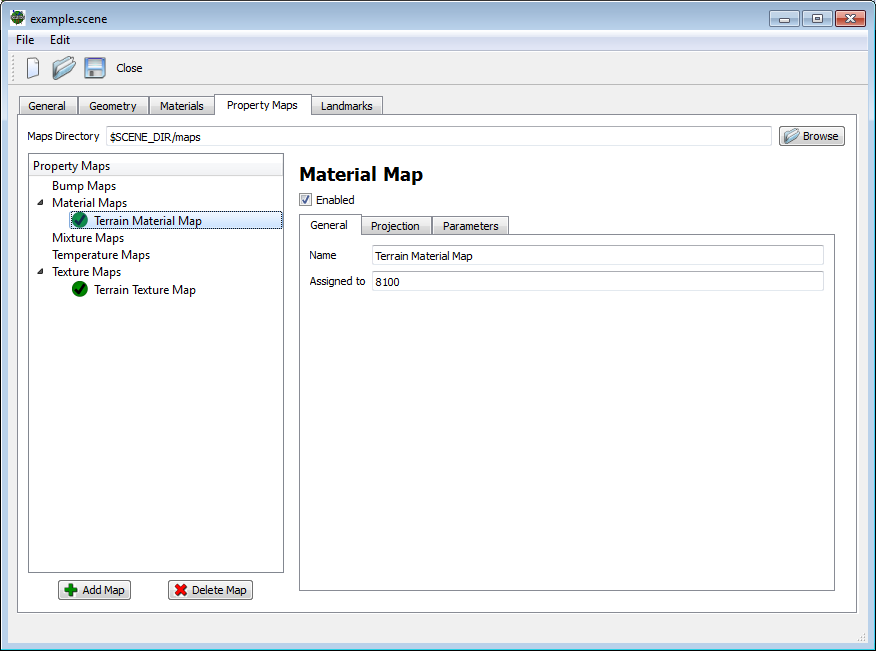
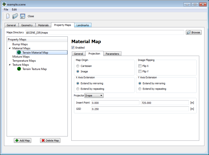
The map list is organized by map type under the Property Maps section of the Scene Editor. From here, the user can set the name, enabled flag, projector, and material ID associations using the tabbed interface provided. To facilitate "bundled objects", maps can also be configured in the material database files. Hence, all map types documented here will show the relevant parts of the graphical user interface in the Scene Editor and the corresponding configuration for the material database file if the map is defined there instead.
Map Types
At this time, there are four general categories of map types:
- Geometry Manipulation Maps
-
These maps manipulate the geometry intersected by the ray tracer before that geometric information is passed to the radiometry model. These maps generally manipulate information including surface normals and surface location.
- Material Manipulation Maps
-
These maps manipulate the materials associated with geometry before that information is passed to the radiometry model. These maps generally handle tasks including remapping materials or mapping multiple materials to a given location.
- Optical Property Maps
-
These maps manipulate various aspects of the optical properties of a given material within the radiometry calculation. For example, introducing spatial variation (also known as "texture") within a given material.
- Temperature Manipulation Maps
-
These maps manipulate the temperature associated with geometry. These maps might manipulate thermodynamic properties used by the temperature solvers or directly inject the temperature solution computed by an external model.
Image Formats
The majority of maps use an image file as input. DIRSIG supports a number of common image formats. There is no need to specify the specific format of the file, it will be interpreted from the format extension, or alternatively from from signature of the file itself. The supported formats (with the standard extension) are listed below:
| Image Format | File Extension |
|---|---|
Windows bitmap |
|
ENVI image |
|
Joint Photographic Experts Group (JPEG) |
|
Portable Network graphics (PNG) |
|
Portable Graymap (PGM) |
|
Tagged Image File Format (TIFF) |
|
X11 pixmap (XPM) |
|
|
|
If you are using a format that supports non-lossless ("lossy") compression, be aware that the individual pixel digital counts may not be what you intended (this can matter for certain maps, such as a material map, where specific digital counts map to specific properties). |
|
|
Maps using an ENVI image file assume that the associated
ASCII/Text header file is available in the same directory.
For example, mixture_map.img and mixture_map.img.hdr.
|
General Properties
Each map has a "name" that is used primarily for documentation purposes (for example, as a reminder of what the map represents). Maps are associate with geometry via material IDs.
|
|
Multiple material IDs can be associated with a single map. This allows the same image file to be shared among maps and minimize memory usage. |
Each map can be enabled or disabled. This feature allows the user to temporarily disable a map rather than deleting the configuration from the scene file.
Map Projection
A map is a 2D image that needs to be associated or projected onto 3D geometry in the scene. At this time, the DIRSIG model provides two projection methods.
-
The drape projection performs a vertical "rubber sheet" projection of the 2D map over the 3D geometry. The major limitation of this projection is the inability to project onto vertical surfaces.
-
The UV projection employs a secondary coordinate system correlated to each 3D geometry vertex in the scene, which allows for maps to projected onto vertical surfaces.
Projection Options
Common to both projection methods is a set of options describing how the source image file is to be mapped from image to projection coordinates and how to handle extension of the image when the projection maps to pixel coordinates outside of the image range.
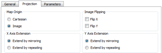
Image Origin
By default, DIRSIG assumes that the origin of an image (either [0,0] in a UV projection or the insertion point in the tile projection) is at the upper left of the image (the vertical coordinate increases going down). However, many tools use an origin that is at the bottom left of an image (vertical coordinate going up). In DIRSIG, we call these two origins Image and Cartesian, respectively (the second coming from the first quadrant in Cartesian coordinates). The user can explicitly choose either of these origins by setting the appropriate attribute to the projection element (see below).
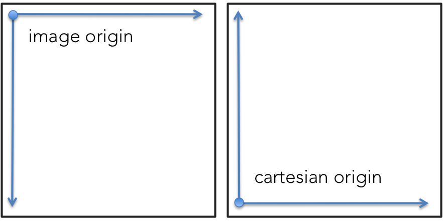
Image Flip
In addition to the the origin assignment, the image can be explicitly flipped across the X or Y axis (or both).
|
|
The Flip Y axis option duplicates much of the functionality of the Image vs. Cartesian image origin option. It is provided for completeness. |
Image Extension
When a given projection method computes a pixel location that is outside the defined image (for example, when the computed image coordinate is (N,0) and the image is only N x M), DIRSIG needs to know how to extend the image. There are currently two options are currently supported:
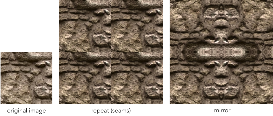
- Mirroring
-
The image is repeatedly flipped about each axis. In a scenario where coordinate (N,0) is requested in an image N x M, the pixel at coordinate (N-1,0) will be used (where the image coordinate in X ranges from 0 to N-1).
- Tiling
-
The image is repeated or tiled for each axis. In a scenario where coordinate (N,0) is requested in an image N x M, the pixel at coordinate (0,0) will be used (where the image coordinate in X ranges from 0 to N-1.)
Both options can be useful for preventing artifacts at the edges of an image. The repeat option is useful if care has been taken to construct a seamless image (i.e. an image that can continuously tile). The mirror options is useful if the image is not seamless since it can create the illusion of a continuous transition (though any structure in the image will create a symmetric structure that is not realistic).
The following sequence of images shows the effect of each type of extension (the seamless image was generated using the GIMP):
Drape Projection
The tile (or "drape") projection simply maps two dimensional pixel coordinates directly to points in the XY plane. There is no vertical component to this map, which results in apparent artifacts on the sides of objects within a scene (e.g. points along a vertical section of a wall in the local coordinate system will have equal [x,y] coordinates, and therefore map to the same pixel even though the z-position varies). That said, this type of map is very easy for mapping terrain properties (materials, textures, etc…) onto a facetized surface generated from a height field.
The tile projection has the important property that it is geometry independent. This can be a useful feature for mapping nadir view imagery onto a terrain model with buildings, roads, etc.., effectively mapping the (top of the) entire scene at once. However, if there is a moving object within the scene such as a car, the geometry will move independently of the map (similar to an object being moved under a tablecloth). Moving objects should always use a geometry based projection, such as the UV projection described below.
In order to position the map within the scene, the user must provide an insertion point in the local coordinate system as well as the size of the pixels on the ground (an effective GSD, or ground sample distance, of the side of a pixel).
|
|
Rotation of the map around the insertion point is not currently supported. The tile projection must align with the XY axes, though there are options to flip the image and change the origin. |
where the Insert Point is in Scene ENU coordinates and the GSD is in meters.
            DRAPE_PROJECTOR {
                INSERT_POINT = 0, 0, 0
                GSD = 0.1
                ORIGIN = IMAGE
                FLIPX = FALSE
                FLIPY = FALSE
                EXTENDX = MIRROR
                EXTENDY = MIRROR
            }
UV Projection
In contrast to the drape projection, the UV projection is geometry based. The columns of pixels in an image are represented on the continuous interval U in [0:1], corresponding to the full width of the image; similarly, the rows of pixels are represented on the continuous interval V in [0,1], corresponding to the height of the image. Every mapped facet in the image is required to have vertex texture coordinates in this UV space that maps that vertex to the image. The UV coordinates of a point internal to a facet is found by applying its barycentric coordinates to the vertex coordinates (i.e. it is a weighted sum of the values at the vertices).
|
|
Texture coordinates and barycentric coordinates for triangles are often described using the same variable names (U and V) which can be confusing. UV texture coordinates are strictly 2D and refer to a position in the image. Triangular barycentric coordinates represent the weights applied to each of the triangle vertexes (usually denoted U, V, and W, also in the range [0,1]). The W is dropped for convenience since W = 1 - U - V. |
3D to 2D Projection via UV Coordinates
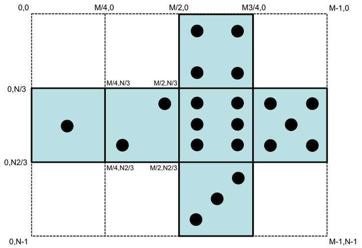
The requirement to use this approach is that the geometry has a UV coordinate system associated with it. This is usually facilitated by an additional 2D coordinate(s) (a UV texture coordinate) that accompany each 3D coordinate in the geometry. The most common example to visualize this relationship is to consider how a 2D map for the faces of a game die would be mapped onto the 3D cube geometry for that object (see illustration below). The 2D map below defines the different faces on the game die. You can see how this map could be printed, cut out and folded up into a 3D cube. In this case, a significant amount of the 2D image space is "empty" (it would have been the scrap if this map was cut out and folded up to make the cube). The coordinates for the face for the "2" side are labeled as fractions of the X,Y dimensions of the image (which range from 0 to M-1 and 0 to N-1 for the X and Y axes, respectively).
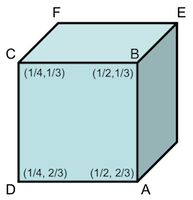
The figure below shows the 3D geometry cube and the 2D UV coordinates associate with the 3D vertexes A, B, C and D on the corners of the front face. Note that each 3D location can have multiple 2D UV coordinates so that the top face (defined by the 3D vertexes B, E, F and C) maps to the corresponding coordinates in the 2D map space for the "5" side.
Because the UV coordinates are fractions, the size of the mapped image isn’t relevant. The UV coordinate is multiplied by the size of the image (in our example, M x N) to get the image coordinates. This also paves the way for multi-resolution images to be used.
|
|
It is possible to have UV coordinates outside of the range [0:1]. In those cases, the map is extended as described by the Image Extension option. This is commonly used when a repeated pattern is desired that conforms to the shape of a geometric object (for example, repeating sections of road). |
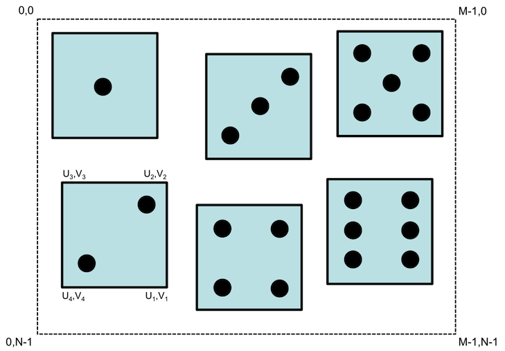
It is important to realize that the 2D map image does not need to resemble the 3D structure it gets mapped to (it does not need to have the property that it can be cut out and folded into the cube). The example below shows another 2D map that is equally valid (but which would require a geometry model that has the corresponding UV coordinates). The only requirement is that the UV coordinates at the 3D corners of each face correctly map to the right regions of the 2D image space.
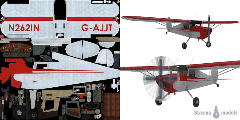
The example below comes from the TurboSquid website, and shows how a complex 2D map can be used to add detail to both internal and external geometry in this model of a Cessna 120:
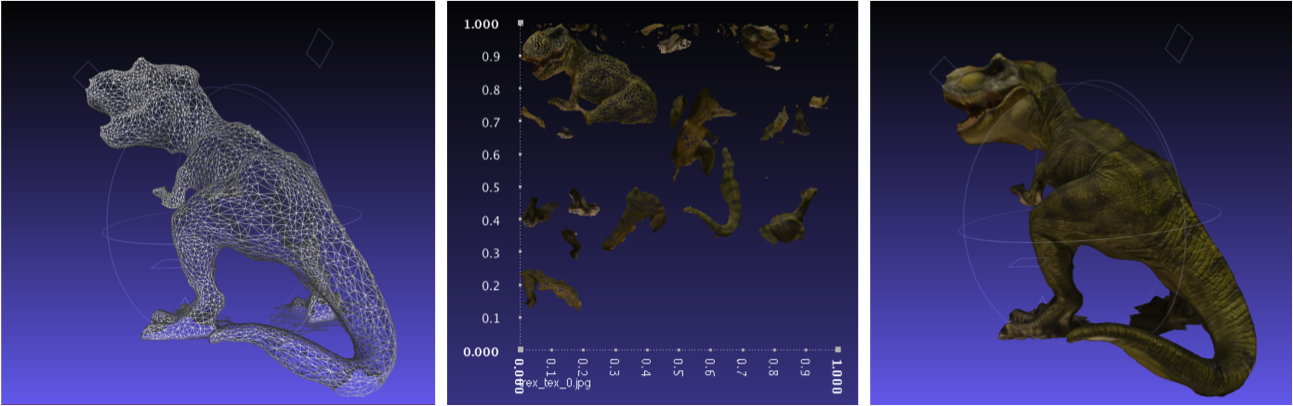
The following sequence of images shows an object with vertex texture coordinates, the image at the locations of those vertexes (and edges) in UV space, and the object with the map applied.
Making UV Wrapped Geometry
Mapping the UV image space to 3D geometry is not a trivial task. There are several commercial and open source tools that can facilitate the process. Most 3D asset generation programs have facilities for mapping 2D maps onto complex 3D models, including Maya, 3d Studio, Meshlab. The details of the process are well beyond the scope of this document. We suggest seeking tutorials for the 3D authoring tool you are using.
Geometry Support for UV Coordinates
UV texture coordinates are only supported by the OBJ geometry format. The DIRSIG specific GDB format does not support UV coordinates. In addition to OBJ files, some of the DIRSIG geometry primitives provide native UV coordinates that can be used. For more information, consult the GLIST documentation.
Projection Configuration
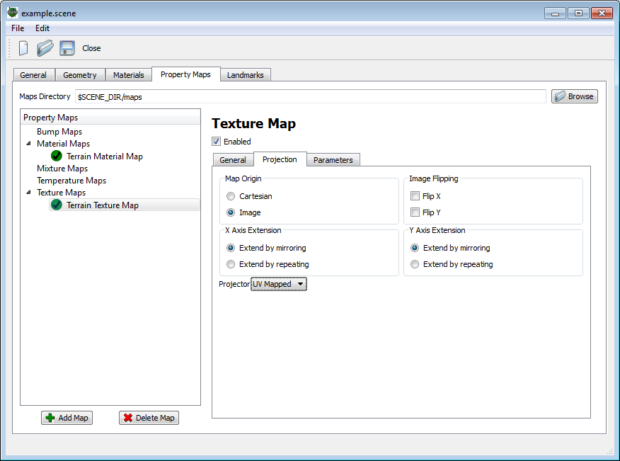
The image below shows a map utilizing the UV projection scheme. Note there are no additional options for the UV projector at this time.
|
|
Prior to DIRSIG 4.5.0, any geometry that contained vertex texture coordinates was forced to use a UV projection (regardless of the projector listed in the scene file). Version 4.5.0 and greater respects the explicit choice of the projector specified. |
            UV_PROJECTOR {
                SPACE = TANGENT
                ORIGIN = IMAGE
                FLIPX = FALSE
                FLIPY = FALSE
                EXTENDX = MIRROR
                EXTENDY = MIRROR
            }
The UV projector supports an additional option that defines what reference coordinate system the map is intepreted in:
SPACE-
The two supported space options are
OBJECTandTANGENT. Since the RGB values in the map explicitly encode the magnitude the normal vector, this option specifies if that vector should be interpreted as being in the coordinate system of the entire object or tangent to the current face. Tangent space maps are frequently used because it means the same map can be applied to different faces regardless of their orientation. Using aTANGENTspace map generally requires the scene model to include explicit tangent data, which can be optionally generated by an option in the GLIST file. The default space isTANGENT.
Geometry Manipulation Maps
The following map types manipulate the apparent geometry of the object intersected before it is handed to the radiometry sub-system for processing.
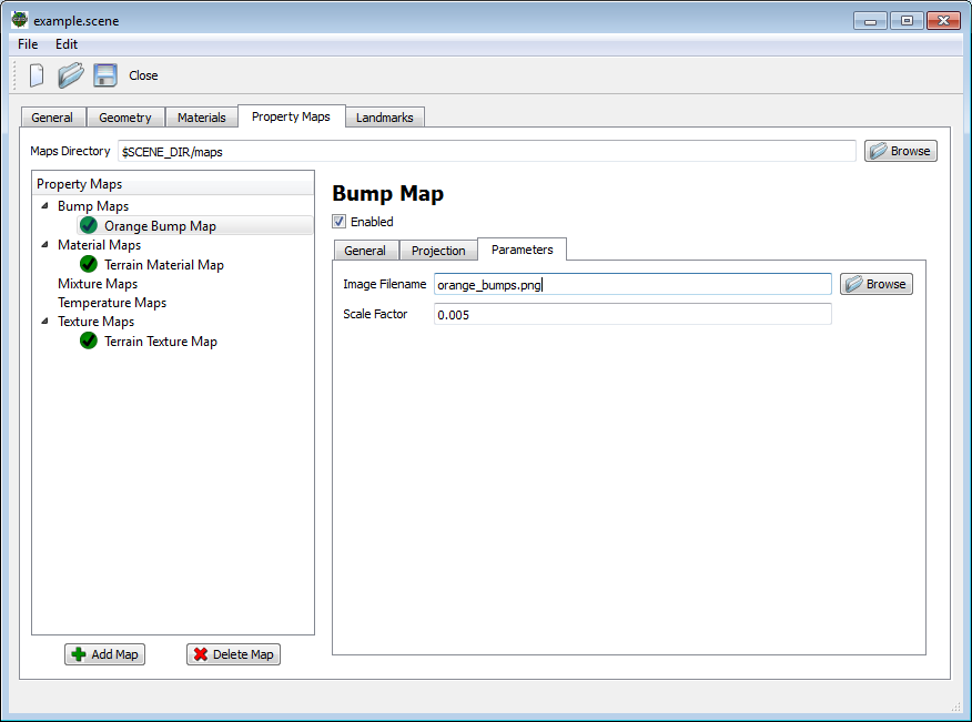
Bump Map
A "bump" map is a common method used in the computer graphics community to introduce apparent surface height variation into smooth surface. The most common example in the literature is to impart the surface height variations of an orange or golf ball onto an otherwise smooth sphere. The technique employs an image map which is used to deflect the surface normal across the surface it is mapped to using gradients in the image. Because the deflected surface normal varies, the leaving radiance of the surface exhibits patterns that mimic what would happen if the surface height (and relative angle to the camera) were actually varying. However, a bump map does not actually displace the surface of the object (it does not "push in" the surface for each golf ball dimple).
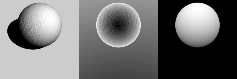
The BumpMap1 demo features an "orange" (as in the fruit) bump map applied to a sphere geometry primitive. The first image below shows the resulting radiance image from the simulation. The shading across the "orange" varies because the bump map manipulates the well behaved normals across the sphere in a way that mimics the surface variations a "real" orange. The middle image is the "normal to view angle" truth image, which shows how the bump map is manipulating the surface normal. The right image shows the average Z intersection truth of each pixel, which highlights that the bump map does not change the location of the surface, but rather the normal at the surface.
The main parameter for the bump map is the scale parameter which manipulates how pixel digital count gradients are translated into surface normal deflections.
Material File Configuration
The option exists to define a bump map in the material database file. To use this option, the user must manually define the material by hand-editing the material database file in a text editor.
MATERIAL_ENTRY {
    ID           = 1
    NAME         = Example
    BUMP_MAP {
        NAME = Bump Map
        ENABLED = TRUE
        IMAGE_FILENAME = orange-bumpmap.png
        UV_PROJECTOR {
            ORIGIN = IMAGE
            SPACE = TANGENT
            FLIPX = FALSE
            FLIPY = FALSE
            EXTENDX = MIRROR
            EXTENDY = MIRROR
        }
        OPTIONS {
            SCALE = 0.005
        }
    }
}
This maps supports the following options in the OPTIONS section:
SCALE-
This variable specifies a scale factor applied to the XY gradient derived from the grayscale map.
|
|
The SPACE option can impact this map type. |
Normal Map
Normal mapping is a technique used to add the appearance of varying surface normals (eg. bumps and/or dents) to a geometric surface that lacks the fidelity required to show these features in the geometry itself. Normal maps differ from bump maps by explicitly encoding the relative normal into the R, G, and B channels of an image.
...
    NORMAL_MAP {
        UV_PROJECTOR {
            SPACE = TANGENT
            ORIGIN = CARTESIAN
            FLIPX = FALSE
            FLIPY = FALSE
            EXTENDX = MIRROR
            EXTENDY = MIRROR
        }
        IMAGE_FILENAME = normals.png
        OPTIONS {
            SCALE = 1.0
        }
    }
...
This maps supports the following options in the OPTIONS section:
SCALE-
This variable can be used to scale the magnitude of the normal map (this parameters in referred to as the "strength" in some modeling tools). The default value is
1.0, a value of0will essentially disable the map and a value greater than1.0will emphasize the map.
|
|
The SPACE option will impact this map type. |
The NormalMap1 demo illustrates the difference between modeling surface topology with normal maps and modeling the same topology with facetized geometry. The NormalMap3 demo includes examples using tangent space normal maps.
Decal Map
A "decal" map is a type of geometry manipulation map that is fairly unique to DIRSIG (to the best of our knowledge). The idea behind it is that we often want to place fairly flat geometry onto other geometry in a way that the first object follows the topology of the second. For example, if our terrain geometry and our uv-mapped road geometry are coming from two different sources (e.g. a DEM and a procedural engine, respectively), it is almost impossible to get the facet edges to map up exactly so that the placed geometry always lies right on top of other.
If the two pieces of geometry are intended to match exactly (e.g. the placed geometry has no depth) then it may be advantageous to only use the underlying geometry and map the properties of the placed geometry onto it (see material and texture maps, below). However, if there is some depth (e.g. a curb) or it is easier to do all the mapping on the placed geometry itself (e.g. if the terrain would require too large a map to reach the desired quality), then the decal map provides a mechanism to generate the desired result.
The decal map works by modifying the position of the mapped geometry so that bottom is always just above the surface it is mapped to. Additionally, the object is rotated so that it aligns with the local tangential plane. The mapped geometry is defined in a GLIST (note that there is no direct ODB support though an ODB can be instanced in the glist) and, like the other maps, is assigned to geometry via a list of material ids. For example, the entry in the scene file should look like:
  <maplist>
    <decalmap name="road" enabled="true">
      <matidlist>
        <matid>4</matid>
      </matidlist>
      <glist>
        <filename>mapped_geometry.glist</filename>
      </glist>
    </decalmap>
  </maplist>
Note that the vertical translation of the object being mapped is ignored — the physical bottom surface is mapped to the underlying geometry.
|
|
Like other property maps, only one decal map is allowed per material. Multiple geometry lists can be placed in the same decal by instancing/including them in a top level glist. |
The DecalMap1 demo shows an example of using this type of map to place a road on a sinusoidal "terrain".
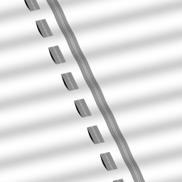
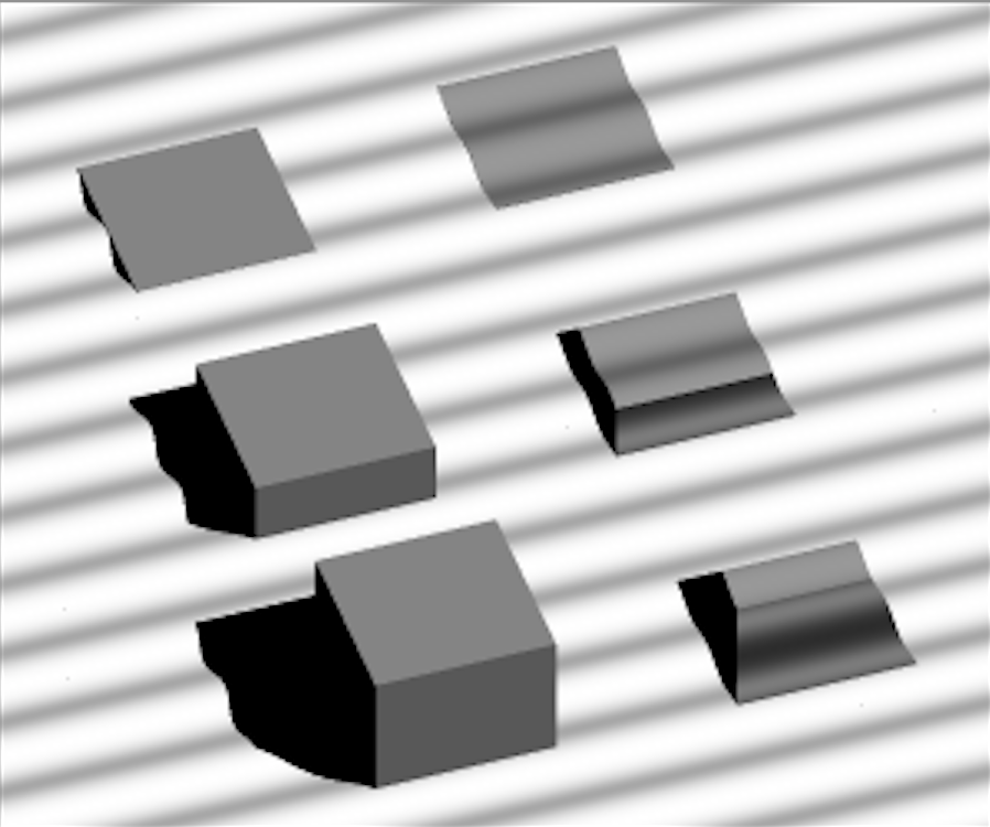
The decal map is only intended for relatively flat geometry. The geometry that is mapped will not cast proper shadows, will not be seen at all angles, and will not maintain the rigidity of objects. For example, the following image shows a box of varying height being decal mapped onto the same sinusoidal surface; the top, shallow box behaves as desired, but with increasing height, the limitations of the map become more apparent.
Material File Configuration
Since the decal map is a geometry concept there is NOT a material map configuration mechanism.
Material Manipulation Maps
The following map types manipulate the material or materials associate with the geometry before it is handed to the radiometry sub-system for processing.
Material Map
The material map is the most commonly used map and associates a class of material (one of the entries in the material database) with geometry. This association is done through a digital count look-up table that matches pixel values to material IDs. Any supported grayscale or RGB image type can be used as input (only the red component is used in the case of RGB images for now).
|
|
A material ID used to associate with a map must always have a definition in the material list (in the case of a material map, that definition will not be used if the map is enabled). |
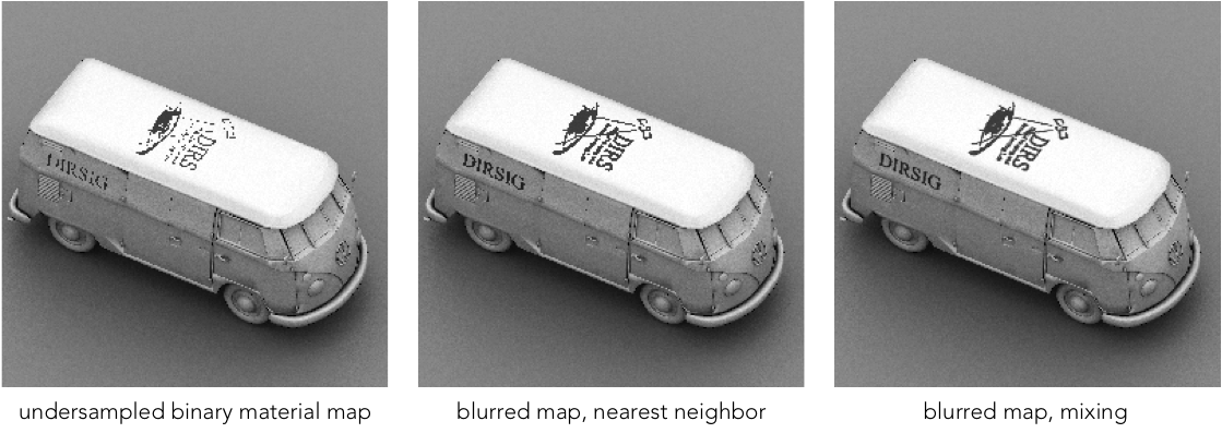
Pure vs. Mixed Mappings
If the pixel value (digital count) encountered in an image is not listed in the look-up table then one of two things can happen. By default, DIRSIG attempts to find a nearest neighbor in the immediate neighborhood of (the specific point within) the pixel with a valid associated material ID. If that fails (i.e. all surrounding pixels do not map to IDs), then the closest defined digital count is used.
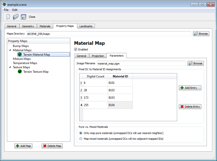
Alternatively, the user has the option to bypass the nearest neighbor search and mix the materials corresponding to the two valid digital counts to either side (above and below the value) of itself. If there is a valid digital count only on one side then no mixing occurs and that material is used directly. This option is very useful for material maps with limited pure materials that have been blurred (low-pass filtered), such as the binary map shown below:
|
|
The mixing option should be used with care since it can double the computation time for every sample encountering that map. |
Material File Configuration
The option exists to define a material map in the material database file. To use this option, the user must manually define the material by hand-editing the material database file in a text editor.
The LUT section contains a list of image digital count and material
label pairs (as a series of DC:Label pairs).
The OPTIONS section contains the only option, which specifies if
mixing should be performed.
MATERIAL_ENTRY {
    ID           = 1
    NAME         = Example
    MATERIAL_MAP {
        NAME = Terrain Map
        ENABLED = TRUE
        IMAGE_FILENAME = materials.png
        DRAPE_PROJECTOR {
            INSERT_POINT = -256, +256, 0
            GSD = 0.24
            ORIGIN = IMAGE
            FLIPX = FALSE
            FLIPY = FALSE
            EXTENDX = MIRROR
            EXTENDY = MIRROR
        }
        LUT {
            6:101
            28:102
            32:103
            173:104
            255:105
        }
        OPTIONS {
            ENABLE_MIXING = FALSE
        }
    }
}
Mixture Map
A mixture map can be used to represent a surface that is a mixture of two or more distinct materials in the material database. The radiometry model computes the surface-leaving radiance for each material and then weights and combines them based on a set of mixing fractions.
|
|
The mixture happens at the leaving radiance level and not at the surface reflectance level. This means that materials in the mixture can use dramatically different surface optical properties and radiometry solvers. It also means that the mixtures behave correctly in the thermal IR, since the relative emission of each material is combined rather than some sort of weighted average material being forged. |
The input to this map is a multi-band image file that contains N bands to define the fractions of N materials at each location. The image file must have the following properties:
-
It must be an ENVI format image file.
-
The weights in each band must range from 0 to 1.
|
|
Weights in the image are not normalized so care should be taken if they are intended to sum to one. |
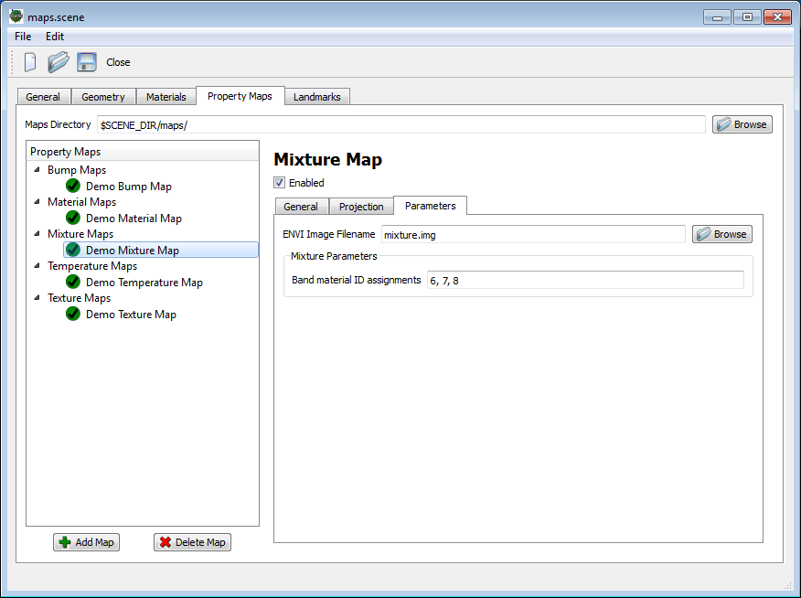
The user must provide the list of material IDs that map to the different
fraction "bands" in the image curve. In the example below, the image file
mixture.img contains 3 bands, with each band containing the fraction of a
specific material for a given location. The Band material ID assignments
list indicates that bands 1, 2 and 3 (or 0, 1, 2) will map to material IDs
6, 7 and 8, respectively.
Material File Configuration
The option exists to define a material map in the material database file. To use this option, the user must manually define the material by hand-editing the material database file in a text editor.
The IMAGE_FILENAME variable points to the compatible ENVI image cube file
containing the material weights (fractions). The BAND_MATERIAL_LABELS
variable is the list of material ID/labels for each band as a common
separated list.
MATERIAL_ENTRY {
    ID           = 1
    NAME         = Example
    MIXTURE_MAP {
        NAME = Terrain Map
        ENABLED = TRUE
        IMAGE_FILENAME = mixture.img
        UV_PROJECTOR {
            ORIGIN = CARTESIAN
            FLIPX = FALSE
            FLIPY = FALSE
            EXTENDX = MIRROR
            EXTENDY = MIRROR
        }
        BAND_MATERIAL_LABELS = water,low,mid,high
    }
}
Optical Property Maps
The following maps manipulate optical properties associated with a material during the surface-leaving radiance calculation.
Texture Map
One of the primary mechanisms utilized in DIRSIG scenes to introduce variation within materials is a "texture map". However, the term "texture map" is generically used in the Computer Graphics community to describe the direct use of an RGB image to define RGB "reflectances" of an object. However, the DIRSIG model must be able to define the reflectances of surfaces at wavelengths outside of the visible RGB region. Furthermore, real materials have specific spectral correlations, where the variations at some wavelengths are correlated to variations at other wavelengths (either positively or negatively). Therefore, a method to introduce spatial and spectral variance was needed.
Algorithm Overview
As hyper-spectral imaging (HSI) systems came into being, a method to simulate these systems was required. Specifically, a method to fuse high spectral resolution point reflectance measurements from field spectrometers (for example, ASD) with high spatial resolution multi-spectral imagery (for example, airborne imagery) was sought. To utilize this method, the following requirements must be met:
-
One or more spatially registered, multi-spectral image bands are needed.
-
A large database of high spectral resolution reflectance curves is needed.
The algorithm initializes itself at the start of the simulation by performing the following calculations:
-
For each image band, the spectral curve database is averaged across the bandpass for that band.
-
The mean and standard deviation of all the curve averages in that bandpasses is computed.
-
The signed standard deviation for each curve average in that bandpass is computed and stored with each curve.
-
-
For each image band, the mean and standard deviation of each pixel in that image is recorded.
When computing the reflectance for a given location, the following process is performed:
-
The digital count (DC) for the mapped pixel is extracted from texture image.
-
The signed standard deviation of that pixel DC is computed using the band mean and standard deviation.
-
The curve in the database with the closest signed standard deviation is used at that location.
|
|
The algorithm does not create new curves on-the-fly. If the spectral curve database only contains 2 curves, then the material will only get mapped with 2 unique reflectances. |
Important notes about the algorithm:
-
Texture map images can be from any wavelength band
-
We commonly use visible imagery because of its availability.
-
-
You can drive the algorithm with more than 1 band image
-
For example, you might have Visible and NIR imagery.
-
The images have to be the same size, registered, etc.
-
The curve that best matches the pixel standard deviations at all the texture driver bands is used.
-
-
You do not need to simulate the same wavelengths as your texture map image.
-
You can simulate the NIR using an image in the visible to drive the algorithm. As long as the spectral curves correctly correlate the variation in the visible with the variation in the NIR, the algorithm will work.
-
In general, the errors increase the farther you get from the texture driver band(s)
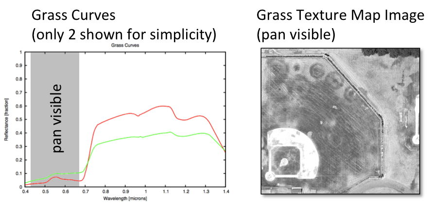
-
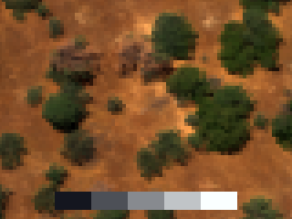
The example configuration below shows how a single panchromatic image (0.4 to 0.7 microns) of grass is being used to drive curve selection from a grass curve database.
Band Statistics Override
The user can override the mean and standard deviation for each texture band image. In some situations the combination of the geometry and the mapping projection will not map all pixels into the scene. Using the mean and standard deviation of all the image pixels might skew the curve selection algorithm (for example, none of the bright pixels might never be used to select curves). This option allows the user to specify the statistics of portion of the image that is relevant.
Material File Configuration
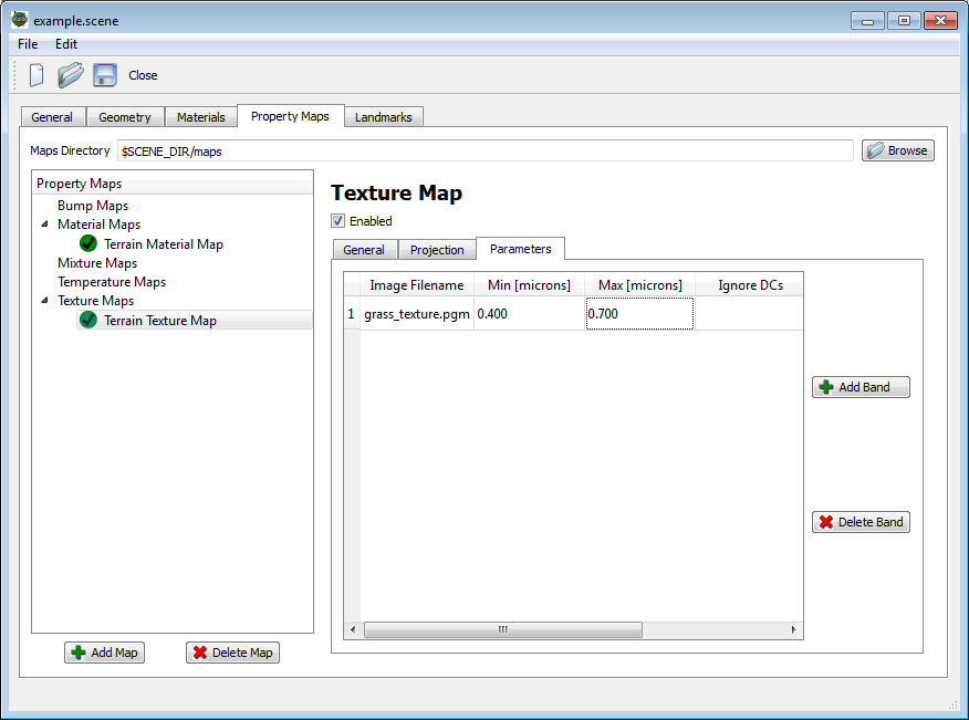
The option exists to define a texture map in the material database file. To use this option, the user must manually define the material by hand-editing the material database file in a text editor.
The IMAGE_LIST section contains the list of images used to drive the
texture algorithm. Each IMAGE section has parameters that mirror the
ones used in a standard texture description. The STATS variable (which
overrides the computed image mean and standard deviation) and IGNORE_DCS
variable (which specifies a list of image digital counts to not include
in the computation of the image mean and standard deviation) are both
optional.
MATERIAL_ENTRY {
    ID           = 1
    NAME         = Example
    SURFACE_PROPERTIES {
        EMISSIVITY_PROP_NAME = ClassicEmissivity
        EMISSIVITY_PROP {
            FILENAME          = emissivity/concrete_texture.ems
            SPECULAR_FRACTION = 0
            TEXTURE_MAP {
                IMAGE_LIST {
                    IMAGE {
                        FILENAME = parking_area.png
                        MIN_WAVELENGTH = 0.4
                        MAX_WAVELENGTH = 0.7
                        IGNORE_DCS = 0,1
                        STATS = 128,30
                    }
                }
                DRAPE_PROJECTOR {
                    INSERT_POINT = -256, +256, 0
                    GSD = 0.24
                    ORIGIN = IMAGE
                    FLIPX = FALSE
                    FLIPY = FALSE
                    EXTENDX = MIRROR
                    EXTENDY = MIRROR
                }
            }
        }
    }
    ...
}
Curve Map
The "curve map" is available as an alternative to the classic DIRSIG texture map approach. Rather than relying on the statistics mechanism of the texture map approach to construct the curve indexes corresponding to digital counts (DCs) in the supplied map image, the curve map interprets the DC values in the map image as the index into the associated curve table. This places the user in charge of creating the curve index image that is used to define where spectral curves will be spatially mapped into the scene.
|
|
This map type is only available in DIRSIG5 and can only be configured as an optical property via the material database. |
Although originally intended to introduce variation within a single material, this map can be used to spatially map curves that correspond to a variety of materials. For example, the spectral database might contain spectral curves for grass, asphalt, concrete, soil, etc. and the map will place those curves into the scene. In this usage, it collapses the conventional material map and texture map hierarchy. However, this unintended usage comes with a few limitations:
-
This mechanism only manipulates the spectral optical property applied at a given location and not the thermodyanmic properties. Only a material map or mixture map can spatially vary the optical and the thermodyanmic properties associated with it.
-
The DIRSIG material truth cannot indicate that some areas were mapped to a curve corresponding to "concrete", "grass", etc. material because the map it does not change the DIRSIG material.
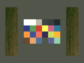
The CurveMap1 demo features a pair of curve map setups. One reproduces the variability one might observe in a patch of grass and the other acts more like a conventional material map by reproducing a Macbeth Color Checker target with a spectral library of curves for they 24 different materials featured in that target.
Material File Configuration
The map configuration includes the following components:
SLI_FILENAME-
The name of the ENVI spectral library (SLI) file containing the spectral curves.
SLI_INDEX_OFFSET(optional)-
This optional offset is added to the digital counts (DCs) extracted from the image file before indexing the spectral library. This makes it easier for large spectral libraries to be shared across mapped materials. For example, two maps might each index 256 curves. Rather than each mapped material using a unique spectral library file containing the 256 curves, a single file containing 512 curves can be used, with first map having an offset of
0(to index the first 256 curves) and the second map having an offset of256(to index the second 256 curves). The default value is0(no offset). IMAGE_FILENAME-
The image file that will be intrerpreted as indexes into the curve library. This image is expected to be a single band image in any of the supported 8 or 16 bits/channel image types, including PGM, PNG, JPEG, and TIFF.
DRAPE_PROJECTORorUV_PROJECTOR-
This section contains variables to control the projection of the image onto geometry.
MATERIAL_ENTRY {
    ID           = 1
    NAME         = Grass (CurveMap)
    DOUBLE_SIDED = TRUE
    SURFACE_PROPERTIES {
        REFLECTANCE_PROP_NAME = CurveMap
        REFLECTANCE_PROP {
            SLI_FILENAME = materials/grass_curves.sli
            SLI_INDEX_OFFSET = 0
            IMAGE_FILENAME = grass_curve_map.png
            UV_PROJECTOR {
                ORIGIN = IMAGE
                FLIPX = FALSE
                FLIPY = FALSE
                EXTENDX = MIRROR
                EXTENDY = MIRROR
            }
        }
    }
    ...
}
The following error conditions are checked:
-
If the image contains a DC that is greater than the number of curves in the spectral library, an out of range error will occur.
Reflectance Map
A "reflectance map" is an optical property that pulls the hemispherical reflectance (HR) from a spectral image file. Although the image file can be a single band or an RGB image, the primary purpose is to allow spectral image cubes (10s or 100s of bands) to be used. The reflectance data is expected to be an ENVI binary data and header file pair. The data should adhere to the following requirements:
-
The band centers should be provided in the ENVI header file (for example,
wavelength = { 0.400, 0.410 ...}).-
If not using an ENVI image, the option exists to specify the band centers within the setup.
-
-
The band units must be microns (for example,
wavelength units = Micrometers). -
The data type doesn’t matter as long as it represents hemispherical reflectances, which should range from 0 → 1.
-
If the user supplies integer or floating point using a range other than [0:1], then a linear scaling can be applied (see the
GAINandBIASoptions) to scale the values into the expected reflectance range.
-
This tool defines the spectral reflectance of a material in the scene. Like all material descriptions, there is no requirement that it use a specific spectral sampling. Hence, the reflectance map image could be sampled on 10 nm centers and other materials driven by spectral curves might be sampled on 1 nm centers. Furthermore, the sensor looking at a material assigned a reflectance map can use any spectral bands to image the material. Any wavelengths imaged outside the spectral range defined by the spectral reflectance image will be flat extrapolated (the closest value within the spectral range will be used).
The ReflectanceMap1 demo features a pair of image files that are used to define the reflectance for two different materials in the scene:
|
|
A reflectance map is not configured via the scene file, but rather in the material file as a surface optical property. |
Material File Configuration
This material can be setup by either manually editing the material database or by using the Custom reflectance property option the Material Editor.
IMAGE_FILENAME-
The name of the spectral reflectance image file.
DRAPE_PROJECTORorUV_PROJECTOR-
This section contains variables to control the projection of the image onto geometry.
BANDS_TO_WAVELENGTHS-
The (optional) comma-separated value (CSV) list of band centers in microns. This option is provided for cases when an ENVI image data+header file pair is not being used. When using an ENVI image data+header file pair, the use of the
wavelengthtag in the header file is strongly encouraged. GAINandBIAS-
The (optional) gain and bias values applied to the image values to scale those values into the expected DHR range of [0-1]. This allows the user to use non floating-point data types for the image data (for example, 16-bit integer data). The default values are
1and0, respectively. CLIP_VALUES-
The (optional) flag to clip values outside of the range [0-1]. The default value is
TRUE. ENABLE_CACHE(DIRSIG4 only)-
The (optional) flag to cache read pixels in memory. If the image is very large, then this can use a lot of memory. However, the image will be queried a lot and the simulation can be slow without the cache in use. The default value is
TRUE. If you observe memory usage issues, then consider changing this option toFALSE. CONVERT_TO_MIXTURE(DIRSIG5 only)-
A reflectance map with only a handful of bands can be alternatively (and more efficiently) represented as a mixture map using internally created spectral curves. A unit reflectance curve is automatically generated for each band plus a "black" (0% reflectance) curve. The map image reflectances are then converted into weigthing factors to linearly mix these curves in order to reproduce the original spectral reflectance from the image. The benefit is a (potentially) significant reduction is storage for a map being represented by a handful of curves and a set of weightings rather than a high spectral resolution image cube.
|
|
Conversion of a reflectance map to a mixture map via the
CONVERT_TO_MIXTURE option is only allowed when the input
image has at most 5 bands.
|
MATERIAL_ENTRY {
    ID           = 1
    NAME         = Grass (Reflectance Map)
    DOUBLE_SIDED = TRUE
    SURFACE_PROPERTIES {
        REFLECTANCE_PROP_NAME = ImageMapped
        REFLECTANCE_PROP {
            IMAGE_FILENAME = grass_refl.img
            DRAPE_PROJECTOR {
                INSERT_POINT = -10.5, -45.5, 0.0
                GSD = 0.25
                ORIGIN = IMAGE
                FLIPX = FALSE
                FLIPY = FALSE
                EXTENDX = MIRROR
                EXTENDY = MIRROR
            }
            OPTIONS {
                GAIN = 0.0000038147
                BIAS = 0.0
                CLIP_VALUES = TRUE
                ENABLE_CACHE = TRUE
                CONVERT_TO_MIXTURE = FALSE
            }
        }
    }
    ...
}
The GAIN in this example is used to scale the 16-bit unsigned values in
the grass_refl.img file down to the [0:1] range expected for reflectance.
In this case, the values in the image file range from 0 to 65,535 and that
maximum value was intended to represent a 50% reflector. Hence, this gain
scales the maximum value of 65,535 to 0.5. The BIAS can be used to
offset the values.
RGB Map
The RGB map feature provided by the RgbImage optical property is
a variation on the reflectance map that pulls
the hemispherical reflectance (HR) from a conventional 8-bits/channel
(PNM, PNG, TIFF, GIF, etc.) image file.
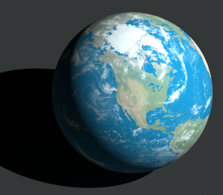
The EarthMap1 demo features a 16200 x 8100 JPEG from the NASA Blue Marble site.
|
|
A RGB map is not configured via the scene file, but rather in the material file as a surface optical property. |
Material File Configuration
This material can be setup by either manually editing the material database or by using the Custom reflectance property option the Material Editor.
IMAGE_FILENAME-
The name of the spectral reflectance image file.
SCALE-
This value is applied to the image values to scale the 8-bit (
0→255) values into the expected DHR range of [0-1]. DRAPE_PROJECTORorUV_PROJECTOR-
This section contains variables to control the projection of the image onto geometry.
MATERIAL_ENTRY {
    ID           = earth_map
    NAME         = Earth Map (via RgbImage)
    DOUBLE_SIDED = TRUE
    SURFACE_PROPERTIES {
        REFLECTANCE_PROP_NAME = RgbImage
        REFLECTANCE_PROP {
            IMAGE_FILENAME = earth_rgb_16k.jpg
            SCALE = 0.00392157
            UV_PROJECTOR {
                ORIGIN = IMAGE
                FLIPX = FALSE
                FLIPY = FALSE
                EXTENDX = MIRROR
                EXTENDY = MIRROR
            }
        }
    }
    ...
}
The SCALE in this example is used to scale the 8-bit unsigned values
down to the [0:1] range expected for reflectance.
Temperature Manipulation Maps
A temperature map takes the place of a numerical temperature solver algorithm and directly manipulates the temperature utilized by the radiometry sub-system to compute the thermal emission.
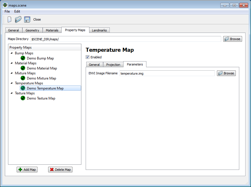
Temperature Map
The temperature map associates a temperature (in degrees Celsius) with geometry. The input to this map is an ENVI image file with a single band. The value of the each pixel in that band is the temperature used.
Material File Configuration
The option exists to define a temperature map in the material database file. To use this option, the user must manually define the material by hand-editing the material database file in a text editor. Under the hood, a temperature map is a temperature solver, so it is specified as such here.
IMAGE_FILENAME-
The name of the image that we be used to drive the temperature solver. This file can be either a floating-point ENVI image file or an 8-bit image file (JPEG, PNG, TIFF, etc.).
DRAPE_PROJECTORorUV_PROJECTOR-
This section contains variables to control the projection of the image onto geometry.
OPTIONS-
This section contains (optional) variables to control the scaling of image values into temperatures. In order to scale the digital counts from an 8-bit image file, the
GAINandBIASvariables can be specified to linearly scale the counts into temperatures. Although a floating-point ENVI image file might contains pixel values that are already in absolute temperature units, theGAINandBIASvariables can still be specified.
MATERIAL_ENTRY {
    ID           = 1
    NAME         = Example
    TEMP_SOLVER_NAME = Map
    TEMP_SOLVER {
        IMAGE_FILENAME = hot_spot.png
        UV_PROJECTOR {
            ORIGIN = IMAGE
            FLIPX = FALSE
            FLIPY = FALSE
            EXTENDX = MIRROR
            EXTENDY = MIRROR
        }
        OPTIONS {
            GAIN = 0.1
            BIAS = 40
        }
    }
    ...
}