GLIST Object Database Format

The primary geometry used by most users in DIRSIG are objects defined by a set of polygons or facets. DIRSIG natively supports attributed, facetized geometry in the following formats:

The base geometry can also be another GLIST or ODB file:

or

And the user can then instance that GLIST or ODB file one or more times into the scene using the same instancing options available for other types of base geometry. This is a mechanism that can be leveraged to easily duplicate large areas of a scene.

A box primitive is modeled using an axis-aligned convention which requires that the user define two corners of the box at the minimum and maximum points (labeled as lowerextent and upperextent, respectively). While this results in a box that is always exactly aligned with the axes of the local coordinate system, the box may be rotated out of alignment using the instance transform.

In addition to the geometric definitions, the user must provide a material ID to apply to the box and has the option of giving a temperature (in degrees Kelvin).

DIRSIG supplies a frustum object that produces a pyramidal frustum with conical corners. The frustum is characterized by sloped sides defined by bottom and top parameters. The bottom takes a width along the x and y axes, a radius, and a center point that positions it in the scene (note that the instance transform must be used to obtain anything other than a vertically (+z) aligned frustum). The top just takes a single radius and is always centered over the bottom. The height finishes off the shape definition and the user supplies a material ID and an optional temperature.

There are a few limits to the types of objects that can be created under this scheme. The bottom radius must always be greater than or equal to the top radius and the width in both axes must be greater than or equal to twice the radius.

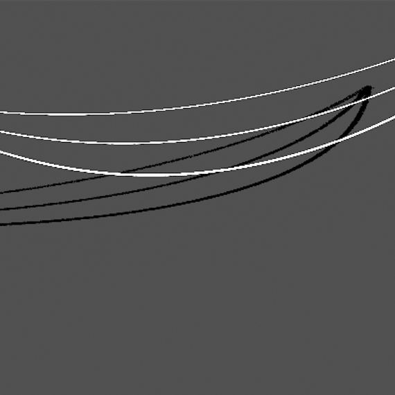
A catenary curve is a hyperbolic cosine function that is a good model of objects strung between two points and sagging under their own weight. Its definition has been simplified as much as possible and requires two points ("a" and "b") and the maximum sag (in meters) between those two points (NOTE: this is not the same as the formal catenary curve sag parameter, which is harder to work with). The user can also set the thickness of the material strung between the two points (assumed to be circular in cross-section) as well as the assigned material. An error will be issued if a curve cannot be generated from the parameters provided. This primitive is particularly good at representing power lines.

The sphere description allows the user to set the center of the sphere, a radius, the material ID and temperature of the object.

A Secchi disk is a high contrast target often used for measuring turbidity in natural waters. DIRSIG provides an easy way to set this up by providing a disk that accepts two materials as input, but is otherwise the same as the disk previously described:

A "regular grid" is a representation of a 3D voxelized field of a spatially varying volume. This data representation is useful for an object like a factory stack plume. The grid description is split between two different files:

The following example shows the contents of a grid file:

The first line has three integers, denoting the dimensions of the grid. In the example above, the grid is 142 x 142 x 64 boxes. The remainder of the file consists of lines with six columns of data. The first three columns indicate the voxel index (counting from 0). The fourth column indicates a DIRSIG material ID corresponding to an entry in the Material Database file (.mat). The fifth column indicates temperature in Kelvin. The final column indicates concentration in parts per million (ppm).

The "grid" file is then inserted into the scene via a GLIST entry like the one shown below:

The <insertpoint> indicates the Scene ENU coordinates (in meters) to insert the origin of the grid (the 0,0,0 coordinate of grid). The parameters <voxeldeltax>, <voxeldeltay> and <voxeldeltaz>, associate a physical size to respective XYZ dimensions of the voxels.

When information in the grid file and the GLIST specification are combined:

A <heightfield> is a 3D representation of a (potentially dynamic) 2D array of height data. It is used in conjunction with a <heightmodel> that defines the heights at each sample point. The model can be as simple as an image (mimicking an unoptimized conversion of elevation data to facetized geometry) or as complex as a wind-driven wave surface that develops over time.

The options to the height field itself are fairly limited:

where <matid> defines the material assigned to the surface (which may be mapped as with other surfaces — the uv space is defined for the horizontal extents of the box height field, with the minimum horizontal point corresponding to the minimum uv point). The two other inputs (<boxmode> and <cachesize>) are optional and rarely used. The <boxmode> uses boxes to model the surface rather than facets. The <cachesize> dictates the maximum number of instantiations of a surface that are held in memory to optimize non-sequential intersection of dynamic surfaces (in particular, this enables faster per-pixel temporal integration). The default values for the two optional parameters are "false" and "100", respectively.

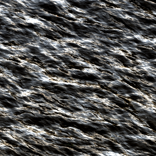
The height field is primarily a way to facilitate bringing regularly sampled height data into DIRSIG without going through an intermediate step of transforming the height data into a facetized 3D object. The advantage of the height field is that all ray tracing is done directly on the height field data itself using an optimized grid traversal algorithm, usually saving both memory and some run time for intersections. This is convenient for static height fields (e.g. terrain) and a necessity for dynamic height fields (e.g. waves)

Internally, the height field is just the grid of data points, with individual surfaces that connect each set of four neighboring points being generated on the fly. This can be seen in a low resolution render using the "box mode", which uses a 3D box at the base of the height field extended to the maximum height of the four neighboring points:

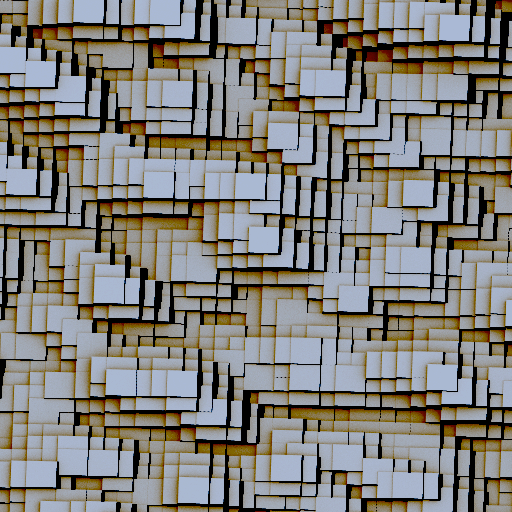
Box mode is only useful under very limited circumstances beyond visualization and normally we want to use the height field in the (default) facetized mode. In this mode, the box is replaced by two triangular facets which collectively have vertices at each of the 4 neighboring data points:

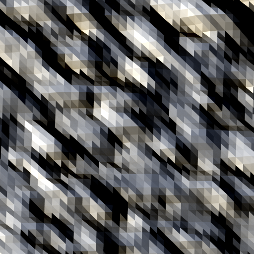
To generate physically realistic scene geometry, the resolution of the grid should be high enough so that the facetization is significantly sub pixel, e.g.

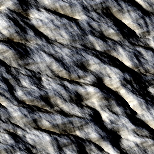
The facetized height field can be treated just like any other facetized piece of geometry — it can be assigned maps and can be given reflectance and transmittance properties:

See the height model documentation for details on how to drive the underlying data.

Using a <pointsource> element as the base source in the GLIST provides the same functionality as the point sources described in Sources without requiring a piece of geometry to define the position, direction and associated material ID. Instead, each point source defined as a base source is always located at the scene origin (it can then be re-positioned using the translation). The default pointing direction is in the positive Z direction, but this can be overridden by rotating an instance or providing an optional new default pointing vector. An element attribute provides the associated material ID and is mandatory:

A "static" instance places the base geometry at a specific location and orientation with the specified scaling. There are currently two ways to define a static instance:

The enabled attribute has been used in some of the previous examples to turn objects and included files on or off in the glist file. The instances themselves don’t have an equivalent input, but it is possible to schedule when they are part of the scene by providing a timewindow attribute,

The time window is a generic term for an on/off schedule and the inputs are dependent on the schedule being used. The type of schedule is automatically determined (the attribute is always timewindow).

Adding more than one <basegeometry> entry to an object allows the user to specify a pool of objects that will be randomly selected from for each instance in the instance list. The different "base geometry" objects can be weighted to create a discrete population distribution that reflects different proportions. The user must still provide a list of instances (either static or dynamic) but the model will choose which "base geometry" is used with each instance based on the weightings. This mechanism can be used for a variety of applications, including:

The different base geometries are defined by creating multiple <basegeometry> elements within an <object> element. Consider the following example from a glist file:

The weight attribute is used to manipulate the relative proportion of that base geometry in the overall population.

In this example, we have defined a pool of four different cars that will be randomly selected from as each instance is defined. Note that the various weight values in this case have the Volkswagen Beetle (vw_beetle.glist) appearing less often than the other vehicles in the scene. It is important to realize that since the vw_beetle.glist file (and the other 3 vehicle GLIST files) include randomized material attributions (discussed in the next section) that each instance will get a random base geometry (which vehicle type) and a random attribution of that base geometry (the paint type on that vehicle).

The ability to randomly reassign material properties to each instance is performed via a <population> element within an <object> element (separate from the <basegeometry> element(s). A <materialvariant> element defines which original material ID will be reassigned and the weighted distribution of assignable material IDs.

In the example below, the model looks for surfaces attributed with material ID #500 (the default material ID for a car, which is associated with the body of the vehicle). These surfaces will be reassigned either material ID #501, #502, #503,#504 or #505 based on the respective weight for each ID. In this case, these material IDs correspond to different vehicle body paints in the DIRSIG material database:

In this case, material ID #501 and #505 have larger weights than the other materials, reflecting that these body colors are more likely to be chosen. The weights add up to 9, which means #501 and #505 will be assigned to 2/9ths (each) of the vehicles and the remaining materials will be assigned to 1/9th (each) of the vehicles.

The simplest form of random fill is based on reading in a list of horizontal positions within the scene and automatically filling them with geometry objects taken from a defined population (see previous discussion of geometry and material variants). For example, we could setup a small fleet of cars (different geometry models with material variants) that looks like this:

Now we can use the new instancing tool to fill the spots listed in one of our lists:

where the options are:

An example of using this fill tool is shown below for a parking lot:

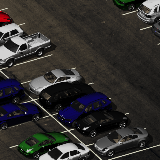
DIRSIG will supply the vertical position (and any slope-based rotation) automatically for the placed geometry based on the underlying terrain/object listed.

We often want to fill an area in the scene somewhat randomly (as opposed to providing a list of locations), but want to have some control over the spatial density of the distribution of objects. Additionally, if there is stuff already in the scene, we potentially want to avoid planting the new object on top of or intersecting those objects (for example, we might want to add a distribution of trees around existing buildings in the scene). The density map (<densitymap>) based random fill is meant to handle these situations:

As seen above, the <densitymap> fill takes a material ID associated with a density map (defined in the maps section of the scene file). The density map (defined in the scene file along with all other maps) might look something like:

The image used for the map is simply a grayscale image where the highest possible value (white) corresponds to the densest packing of objects and the lowest possible value (one digital count above black) corresponds to the least dense packing. A value of zero (absolute black) in the image means that no objects should be planted in that region (which is useful for masking out portions of the scene where objects would be planted otherwise).

The practical definition of density is based on the provided values for <mindist> and <maxdist>. These values are approximately the spacing between the placed object at the highest and lowest density, respectively (they are actually the distances between the transformed bounding boxes of the placed objects since it would be too expensive to test potentially complex surfaces). When two objects exist in two different density regions (e.g. two different points in a density gradient) then the distance between them will be the average of the two density based distances.

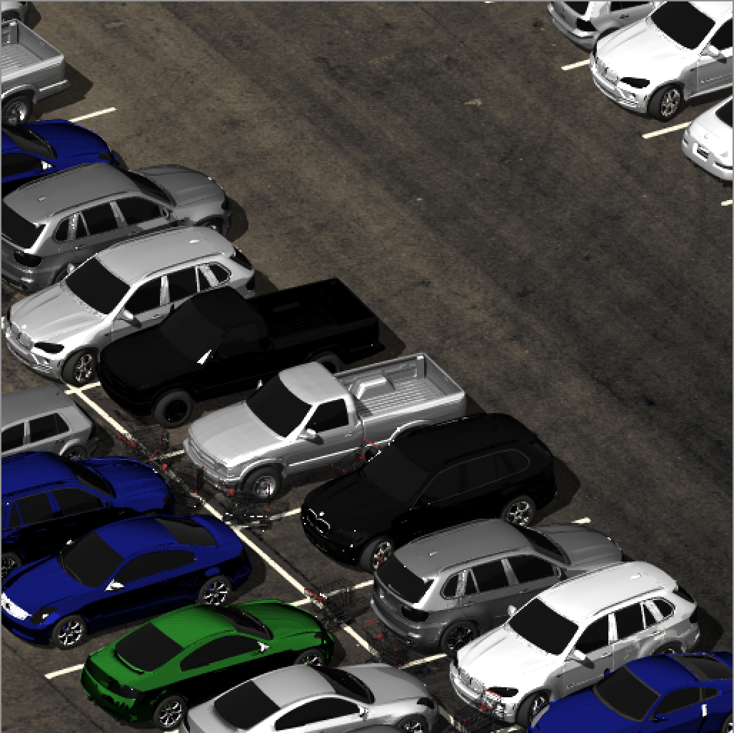
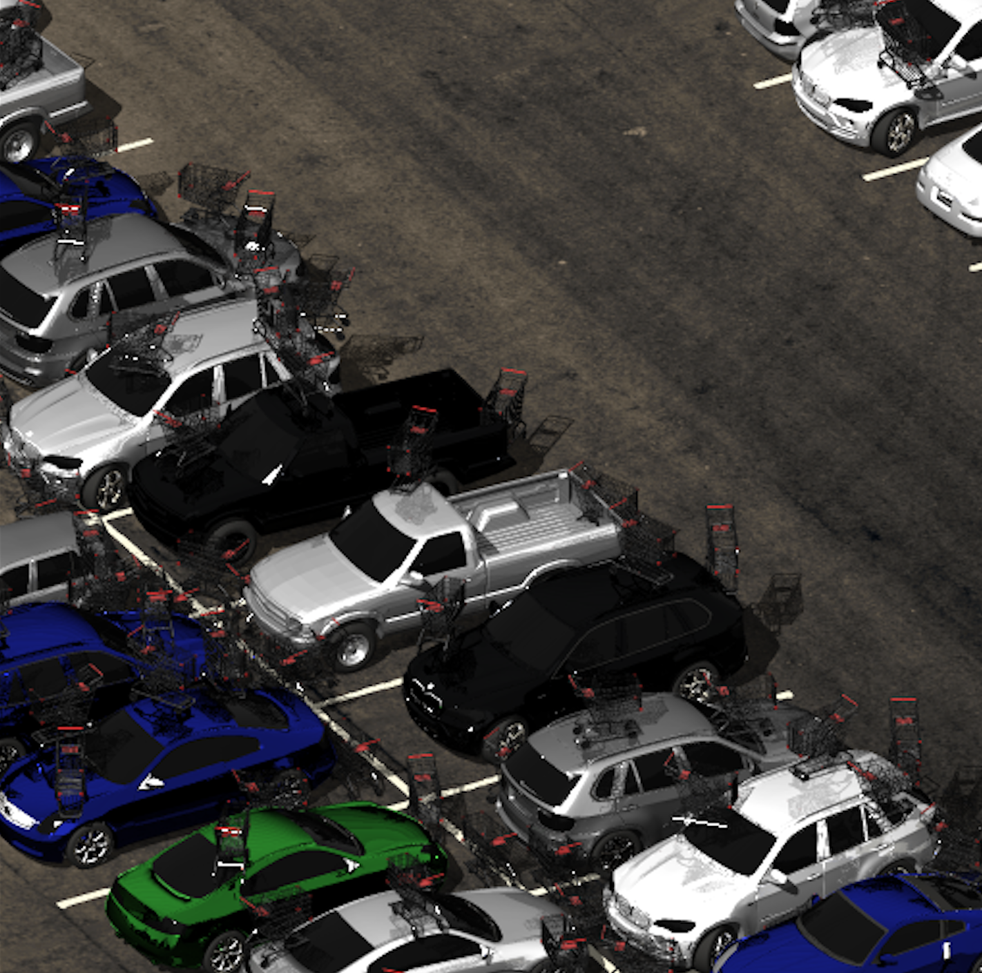
The following image is an example of using the density map to place stray shopping carts in a grocery parking lot scene in a semi-logical fashion (i.e. in between cars, and primarily between opposing stalls, but never in the drive aisles).

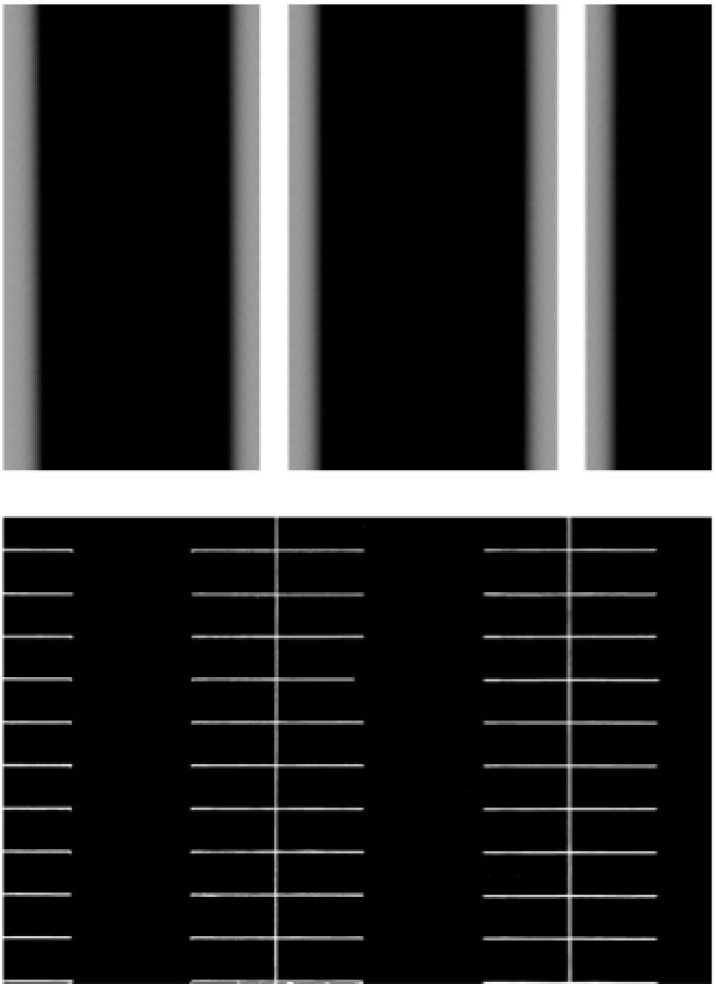
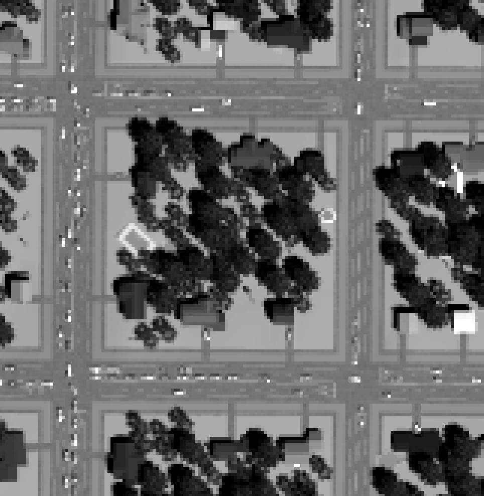
The density map we’re using (shown below, above the material map that defines the lines) shows how this was done. The area between opposing stalls has a band of pure white (highest density packing), the areas between cars have a darker value with a slight gradient (we want a few carts between vehicles, but make it very unlikely to pack two in close together), and finally the drive aisles are black, making sure there are no carts blocking traffic.

The other key part of the <densitymap> is the choice of <anchor>, which is that name of a (unique) geometry instance in the scene. This the object onto which the objects will be placed. If the anchor is occluded by another object (e.g. a car on the parking lot when the lot is the anchor), then the object won’t be placed. Otherwise each placed object will rest on the anchor object based on its "origin" (usually set to the center bottom of the object).

Note that our choice of anchor is important here (it was assigned to the parking lot geometry instance, "lot"). If the entire scene was used as the anchor then carts would be placed where ever they fell (though avoiding each other). The following image shows this (for a larger number of carts than used in the previous):

The <anchorlist> and <densitymap> fills are used in the Parking1 demo which was used to create the images shown here.

The polygon (vertex) based fills are setup similarly to the density based fill except that objects are placed uniformly within each polygon:

with options:

The following image is an example of using backyard polygons to direct the placement of tree, pool, and playground clutter (note that there is no socio-cultural logic applied — a pool is placed near a sidewalk even though that would not be likely to occur):

There is nothing stopping you from creating multiple GLIST files in a given bundle folder. For example, the Infinity G35 example above creates a bundle for that car painted blue. The bundle material file (in this case infinity_g35.mat) could also have entries for red, green, white, etc. paint and the materials folder can contain the various spectral optical property files for those materials. Then you can create multiple GLIST files, each with a unique paint scheme by changing the <assign> elements to map to the desired paint material to the body. This allows you to easily create bundles of the same geometry (the OBJ file does not need to be unique) with multiple attribution schemes.

Since the "entry point" for a bundle is standard GLIST file, there is no reason why that GLIST file cannot contain multiple <object> entries. The BundledObject2 shows how an object can been combined with other objects in the bundle GLIST. In that case, various sources are combined with an OBJ file.