This document describes the basics of creating user-defined point sources (sometimes called "secondary sources") in DIRSIG. These point sources can be assigned spectrally varying emission functions and can use angular weighting descriptions to focus or shape the output.
Description
Point sources are modeled by creating a special geometric description and associating a specific material description with that geometry.
|
|
Point sources can now be directly viewed by a sensor, but see the explanation below to understand the approximations that go into the radiometry to do this. |
Geometry Description
A point source is placed in the scene via a special geometric description. There are two ways to define the location and orientation (pointing direction for a shaped source) of the source:
-
As a special object type in a geometry list (GLIST) file. This is the preferred method.
-
As a single vertex facet (polygon) in a geometric database (GDB) file. This is the older method with several limitations.
The Geometric List (GLIST) Method
The preferred method to define the geometry of a point source is via the
<basesource> description in the GLIST
file. There are several benefits to using the GLIST approach:
-
The specialized source geometry is not in a standard geometry file used for 3D content creation/editing tools that generally don’t have standardize descriptions for such elements.
-
The GLIST file allows sources to be easily instanced, both statically and dynamically.
Below is a simplified version of the
geometry/bundles/police_car/police_car.glist file in the
BundledObject2 demo.
It shows how to craft a GLIST file that mates a OBJ file for a car with
a pair of headlights:
<geometrylist>
  <object>
    <basegeometry>
      <obj><filename>nissan_march.obj</filename></obj>
    </basegeometry>
    <staticinstance/>
  </object>
  <object>
    <basesource>
      <pointsource matid="headlight">
        <pointing><vector><x>0.0</x><y>1.0</y><z>0.0</z></vector></pointing>
      </pointsource>
    </basesource>
    <staticinstance>
      <translation>
        <point><x>-0.66</x><y>1.6</y><z>0.7</z></point>
      </translation>
    </staticinstance>
    <staticinstance>
      <translation>
        <point><x>+0.66</x><y>1.6</y><z>0.7</z></point>
      </translation>
    </staticinstance>
  </object>
  ...
<geometrylist>
The first <object> is the OBJ for the car. The second <object> is
the headlights for the car. The base source is created with a direction
vector pointing in the +Y direction, since that is the direction the front
of the car is facing. This source is then statically instanced twice — once for each headlight. Each instances has the relevant +/-X offset to
position the headlight on the driver and passenger side, the same +Y
offset to position the source just in front of the car, and the same +Z
offset to raise the source to the proper height.
|
|
As a reminder, material labels (IDs) in DIRSIG do not need to be
numerical. A unique, alpha-numeric label can make it much easier to
manage a large set of labels (IDs). In this case, the material
label we chose was headlight.
|
With this GLIST configuration, the base geometry for the car can be modified in a variety of ways. The setup will continue to work as the OBJ is updated as long as the position and size of the car doesn’t change, which would mean the headlight instances would need to be updated.
The Geometric Database (GDB) Method
The approach to defining a point source in a GDB file is to create a single-vertex polygon (essentially a point) and to use the explicit normal in the GDB file to define the pointing direction. There are several limitations to using the GDB approach:
-
The geometry description must be created by hand since the popular 3D content creation tools do not provide methods for creating single-vertex polygons (anything less that three vertexes is usually considered degenerate geometry).
-
Likewise, you cannot load a geometry file that includes a point source described by a single-vertex facet into Bulldozer, Blender and other 3D authoring tools because, again, most tools consider a single-vertex, zero-area facet (polygon) invalid.
|
|
Point sources cannot be described in Alias/Wavefront OBJ files because the single-vertex facet needs an explicit normal vector to define the source direction and OBJs employ implicit normals described by the vertex order. |
However, this approach was used in older versions of DIRSIG4 and some of the demos still employ this approach to insure we have regression test cases.
The following is an example GDB file containing a
single facet that is a source. The source is located at 5, 5, 10
and is pointed directly "down" (0, 0, -1). Notice that the facet
description contains a single vertex indicating the sources description
and the normal indicating the desired down direction. The radiometric
properties of the source will be described by the material with ID
2669K_omni_source.
|
|
As a reminder, material labels (IDs) in DIRSIG not not need to be numerical. A unique, alpha-numeric label can make it much easier to manage a large set of labels (IDs). |
OBJECT
PT_SOURCE_OBJECT
1-0-0
PART
PT_SOURCE_PART
1-1-0
FACE
PT_SOURCE_1
1-1-1
PointSource
2669K_omni_source
NONE
0.00
1.0000
0.0000
0.0
null
null
null
1
5.000000000000000e+00 5.000000000000000e+00  1.000000000000000e+01
0.000000000000000e+00 0.000000000000000e+00 -1.000000000000000e+00
0.0000000000
0.0000000000
0.0000000000
END
A GDB containing a source can contain other non-source geometry. For example, the GDB for a truck might have two source facets (one for each headlight) that point forward. Or a street light GDB might contain the geometry for the lamp post and a single facet for the "bulb" that points down. However, at RIT we frequently place source facets in a separate GDB file so that the source geometry (single vertex facet) does not render the entire file "invalid" (most tools will treat a single-vertex, zero-area facet as invalid) when trying to load it in a 3D authoring tools such as Bulldozer and Blender.
Material Description
The geometric description of the point course is assigned a material
that describes the radiometric properties of the course. An
appropriate entry must be made in the Material Database
file (.mat). A source material description is different than a
conventional surface or volume material. This description consists
of the following components:
-
Radiant intensity filename (see the INT file format)
-
Optional shaping description
-
Optional normalization flag
-
Optional blinking or modulation description
The following is an example source material entry:
MATERIAL_ENTRY {
    NAME = 2669K, omni-directional point source
    ID = 2669K_omni_source
    OPTICAL_DESCRIPTION = SOURCE
    INTENSITY_FILENAME = 2669K.int
    SOURCE_SHAPE = 0.0
    NORMALIZE_SHAPE = TRUE
    EDITOR_COLOR = 1.0, 1.0, 1.0
}
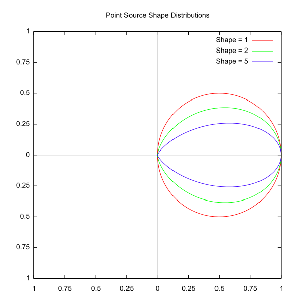
Shape Coefficient
By default a point source is omni-directional, radiating equally in all directions.
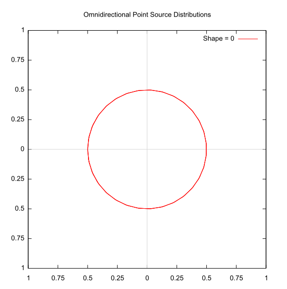
However, the user can specify an optional shaping coefficient
that can "focus" the output of the source into a given direction
using the SOURCE_SHAPE variable. The "focused" illumination
pattern is directed into the direction indicated by the explicit
normal vector provided in the geometric description of the point
source. This coefficient is the exponent applied to a cosine
shaping function:
\(I(\theta, \lambda) = \Omega(\lambda) \cdot \cos^n(\theta)\)
where I is the radiant intensity in Watts/(sr micron) into the angle direction theta at wavelength lambda, O is the spectral radiant intensity curve from the INT file and n is the shaping coefficient.
|
|
The default SOURCE_SHAPE value is 0.0, or an omni-directional
distribution.
|
In DIRSIG5, a feature was added that allows the user to supply a
weighted combination of shapes via the SHAPING_LIST section. In lieu
of a single SOURCE_SHAPE variable, this section is provided as a
set of shape and magnitude pairs:
    SHAPING_LIST {
        SHAPE_MAG_PAIR =  1.0,0.2
        SHAPE_MAG_PAIR = 20.0,0.8
    }
See the Sources5 demo for more information.
Normalization Flag
As you can see from the plot of the shape coefficients, the total
area within the radial distribution is dependent on the shape
coefficient. This creates a issue where the total radiant intensity
(integrated over all angles) described by the INT file
is not preserved with shape coefficients greater than 1. The
NORMALIZE_SHAPE variable allows the user to force the shaped radial
distribution to be weighted so that the total radiant intensity is
preserved.
|
|
For the 4.5.1 release, the default NORMALIZE_SHAPE value was
changed from FALSE to TRUE. Since many old scene setups do
not have this flag in them, the results from 4.5.1 and newer
releases will be different than simulations performed with
4.5.0 or older. If the NORMALIZE_SHAPE flag is present,
then the results should not vary with release.
|
Blinking Sources
By default a source is continuous (constantly "on"). However,
there are two options to model a non-continuous source. The first
option is a blinking source that turns on and off at a user-supplied
frequency. The on/off pattern consists of instantaneous on/off
transitions. This is enabled by setting the corresponding on/off
frequency (in Hertz) and an optional temporal offset for the on/off
pattern to start (in seconds) in the material description via the
BLINK_FREQUENCY and BLINK_OFFSET variables, respectively:
    BLINK_FREQUENCY = 20.0
    BLINK_OFFSET = 0.0
Modulated Sources
The second option for a non-continuous source is a modulated source, which varies in magnitude according to a user-supplied power spectral density (PSD) curve. Below is an example of an XML-formatted PSD file:
<psd frequencyunits="hertz">
  <entry>
    <frequency>0</frequency>
    <magnitude>2.5</magnitude>
    <phase>0.00000000</phase>
  </entry>
  <entry>
    <frequency>2000</frequency>
    <magnitude>2.5</magnitude>
    <phase>0.00000000</phase>
  </entry>
</psd>
The frequency is always in Hertz, the magnitude is unitless and the phase is always in radians.
Each <entry> in the file defines a frequency mode, with a unique
magnitude and phase. The modulation for each frequency entry will
produce positive and negative values. The magnitude at any given
time is computed as the absolute value the summed magnitude of
all the frequency entries.
|
|
As many frequencies can be defined as you wish, however there is a computation advantage to not specifying trivial frequencies with very small magnitudes. |
To create a frequency modulated source, the name of the PSD file is
provided in the material description via the PSD_FILENAME variable:
PSD_FILENAME = 60Hz.psd
Both of these options are featured in the Sources4 demo.
Directly Viewing Point Sources
Point sources, by definition, subtend a solid angle of zero from any view direction. This poses a problem for directly viewing a source under a ray tracing modality since the pixel solid angle (or portion thereof) that the ray represents will never "see" the source and there is no explicit surface to calculate the incident flux upon.
To approximate the expected effect of a point source, we add in a contribution from each source that falls within the solid angle of a pixel ray. That contribution is based on treating the source as if the distribution integrated by the solid angle is a Dirac delta function, such that the integrated radiance into the ray solid angle is equal to the magnitude of the intensity into the direction of the ray origin. Since the radiance required by DIRSIG as a solution for that ray is distributed over its solid angle, we weight the source integrated radiance by the inverse of that angle.
Transmission between the source and the sensor is also taken into account, and the rest of the solid angle is calculated as usual by sampling the scene (since the solid angle of the source is still zero, we don’t have to worry about the source blocking a portion of the scene).
|
|
To make this process computationally efficient, testing for an overlap between the ray solid angle and the source is done by checking the relative angle between the ray and a source vector. The check is based on a circular cross-section that circumscribes the ray solid angle (which is assumed to be square in cross-section). Since the test is slightly larger than the actual solid angle, there can be overlap between pixels that does not exist when the source is near an edge and the sensor effective response is ideal. Additionally, the assumption of a square solid angle may not be true (pixel can be rectangular) and may create additional artifacts. |
Using Real World Descriptions
The DIRSIG model ingests radiometric descriptions for user-defined sources. However most sources in the "real world" are described using terms including "total power", "luminous efficiency", etc. This section attempts to explain how these real world descriptions can be used to drive DIRSIG simulations.
Total Integrated Power
To compute the total integrated radiant power from a DIRSIG radiant intensity (INT) file, the file must be integrated over the surface of a sphere (the file nominally represents the radiation going in all directions) and all wavelengths:
\( \mathrm{Total~Radiant~Power} = \oint \int\limits_{\lambda_1}^{\lambda_2} I( \lambda ) ~d\lambda ~d\Omega ~\mathrm{Watts} \)
Photopic Response
Since real world sources are primarily employed to aid in human vision, most source descriptions are in terms of luminous flux (which incorporates the response of the human visual system) rather than radiant flux. The luminosity function (F) describes the (average) spectral sensitivity of human visual system to spectral radiance as a function of wavelength:
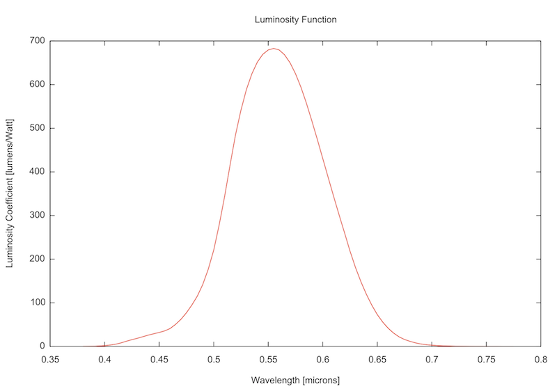
Brightness
To get the total photopic power or brightness, the total radiant power integral must incorporate the luminosity function:
\( \mathrm{Brightness} = \mathrm{Total~Photopic~Power} = \oint \int\limits_{\lambda_1}^{\lambda_2} F( \lambda ) ~I( \lambda ) ~d\lambda ~d\Omega ~\mathrm{lumens} \)
Luminous Efficacy and Efficiency
Most sources only radiate a portion of their energy at wavelengths overlapping the human visual system. For example, most broad-band sources (incandescent) have a significant amount of energy emitted in the infrared regions (most sources of this type convert only about 10% of their input energy to visible light). The terms luminous efficacy and luminous efficiency are often employed to describe how much of the spectral energy generated by a source is in the response region of the human visual system. The luminous efficacy is the ratio of the total photopic power (brightness) and the total radiant power:
\( \mathrm{Luminous~Efficacy} = \mathrm{\frac{Total~Photopic~Power}{Total~Radiant~Power}} = \frac{ \oint \int_{\lambda_1}^{\lambda_2} F( \lambda ) ~I( \lambda ) ~d\lambda ~d\Omega} { \oint \int_{\lambda_1}^{\lambda_2} I( \lambda ) ~d\lambda ~d\Omega} ~\mathrm{lumens/Watt} \)
The luminous efficiency is the ratio of the luminous efficacy to the maximum luminous efficacy of 683.002 lumens/Watt.
\( \mathrm{Luminous~Efficiency} = \mathrm{\frac{Luminous~Efficacy}{683.002}} \)
Electrical Efficiency
Neither the luminous efficacy nor the luminous efficiency values explicitly convey information about how much of the electrical energy input to the source was converted to radiant energy. In some cases it is assumed that the any electrical power that is dissipated as heat (for example) is captured in the total radiant intensity.
|
|
The luminous efficacy and luminous efficiency do not carry information about the electrical efficiency of a source. They only convey the spectral overlap of the emitted radiance and the human visual response. |
Example Source Characteristics
The table below contains luminous efficacy and brightness values for common sources: [1]
| Electrical Wattage | Efficacy (lumens/Watt) | Brightness (lumens) |
|---|---|---|
40 W tungsten incandescent |
9-12 |
360-500 |
60 W tungsten incandescent |
12-15 |
720-900 |
75 W tungsten incandescent |
14-16 |
1050-1200 |
100 W tungsten incandescent |
12-18 |
1200-1800 |
150 W tungsten incandescent |
15-20 |
2250-3000 |
200 W tungsten incandescent |
16-20 |
3200-4000 |
300 W tungsten incandescent |
18-21 |
5400-6500 |
Low pressure sodium (LPS) and high pressure sodium (HPS) lamps are commonly used in urban lighting applications for streetlights. An LPS bulb can have an electrical wattage of 10 to 150 Watts and an efficacy of 100 to 150. Unlike the broad spectrum generated from most incandescent bulbs, LPS bulbs generally have a narrow emission spectrum centered at 589.3 nm and are therefore recognized by a pure orange color. In contrast, an HPS bulb uses high pressure gas (to induce pressure broadening in the sodium emission) and other metals (including mercury) to create a broader spectral coverage than LPS bulbs. These bulbs are usually perceived as having a pinkish orange color. An HPS bulb has a typical electrical wattage of 50 to 1000 Watts and an efficacy of 100 to 150 (higher values for higher wattage bulbs).
40 Watt Incandescent Example
Consider the 40w_2700k.int file included in the Sources1 demo, which
has the following characteristics:
-
The total radiant power is 40 Watts
-
The brightness is 496 lumens
-
The luminous efficacy is 12.562 lumens/Watt
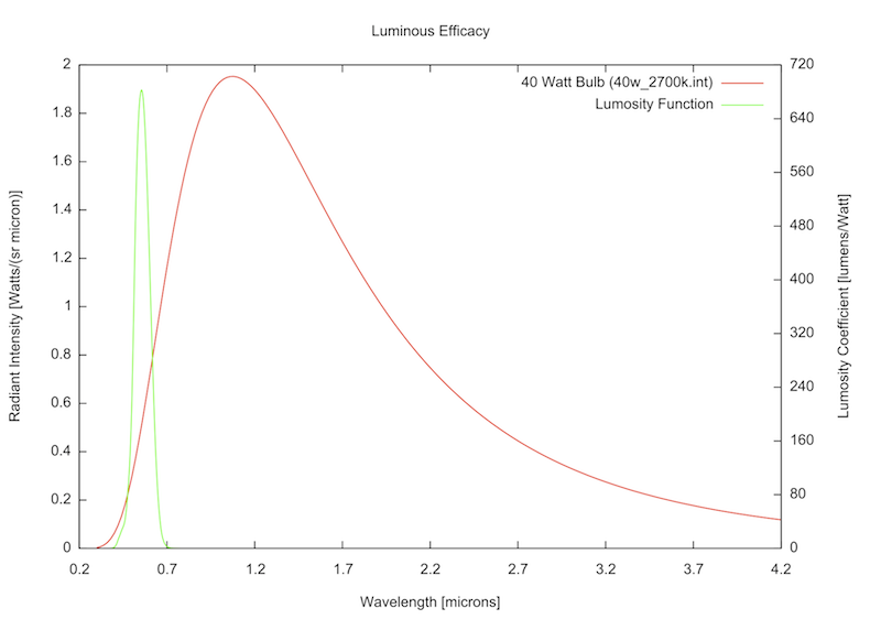
The luminous efficacy and brightness corresponds well to a "40 Watt tungsten incandescent" source in the table above.
Relevant Options (DIRSIG4 only)
There are several options available for fine tuning the behavior of the
secondary source radiometry solver (responsible for all indirect
contributions from the source). Currently, these are set via the
.options file.
|
|
These options are only relevant to DIRSIG4. |
Disable Sources
By default the contribution of user-defined is always considered. However,
in some cases the user may wish to disable these contributions. For
example, to turn off all the lights in a scene at night or to ignore all
the lights in a scene during the day. A single, central option is
available to disable all user-defined source contributions (via the
secondarysources.disable entry) and the default value for this option
is false.
Rejection Threshold
When scenes are spatially large and/or there are a large number of sources, computing the contribution from every source can be can lead to excessive run-times. Therefore a contribution rejection mechanism is used to ignore the contributions from sources that are expected to not make significant contributions to the radiance reflected by a surface.
Starting in DIRSIG 4.6, a sorting mechanism was introduced to setup
an internal grid-like map that allows the model to only consider sources
within a given area that will contribute significantly. This threshold
drives which sources are considered important as a function of position
in the scene. The image sequence below was created using the Sources1
demo, and shows how the threshold can impact the results. In this example,
the source is a modest 40 watt bulb that is 5 meters from an 18% reflector.
The default threshold (1.0e-05) considers the reflected radiance from
this source to be insignificant, and ignores that sources (left image).
The center image overrides the threshold with a value of 1.0e-06, which
considers the contribution significant near the source, but it does not
meet the threshold within the internal grid sorting as we get father away.
The right image employs a threshold of 1.0e-07, which is low enough that
the source is considered significant everywhere within the field-of-view.

|
|
The image viewer is using a high gain scaling to show how this threshold impacts the simulation. The square cutoff in the center image reflects the source being ignored after it has dropped nearly 2 orders of magnitude from the peak value. In terms of absolute radiance, this specific source’s contribution might be well below the noise or quantization limits of your sensor. Therefore, the value of your threshold is very application specific. |
This threshold can be manipulated in the options file via the
secondarysources.threshold entry. The default value for this option
is 1.0e-05.
|
|
We are exploring ideas to make this threshold dynamic, such that it could adapt to a scene with a lower light level automatically. |
Direct Viewing
Direct viewing of a source (discuss previously) is controlled in the
.options file via the secondarysources.viewdirect entry. The default
value for this option is true (sources are directly viewable).
Other Options
secondarysources.samples-
The maximum number of samples to use integrate sources with volume. The default value for this option is 250.
secondarysources.shadowquality-
A scalar between
0.1and1.0that drives how long DIRSIG takes looking for soft shadows before assuming that its hard. The default value for this option is 0.25.
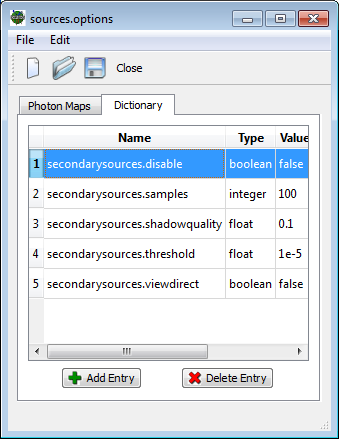
Example Options File
The following example shows these variables being manipulated
in a DIRSIG Options Editor (see the Dictionary tab) or directly
in the .options file:
<options>
  <dictionary>
    <entry>
      <name>secondarysources.disable</name>
      <type>boolean</type>
      <value>false</value>
    </entry>
    <entry>
      <name>secondarysources.samples</name>
      <type>integer</type>
      <value>100</value>
    </entry>
    <entry>
      <name>secondarysources.shadowquality</name>
      <type>float</type>
      <value>0.1</value>
    </entry>
    <entry>
      <name>secondarysources.threshold</name>
      <type>float</type>
      <value>1e-5</value>
    </entry>
    <entry>
      <name>secondarysources.viewdirect</name>
      <type>boolean</type>
      <value>false</value>
    </entry>
  </dictionary>
</options>
Options Dictionary Editor
The following example shows the relevant sources options being manipulated in a DIRSIG Options Editor (see the Dictionary tab).
|
|
Options in the Options Editor Dictionary do not appear in the automatically. They must be manually added at this time. |
Relevant Demos
The following demos can be explored for specific examples of point and extended source scenarios:
-
The Indoors1 demo contains a single point source illuminating an "indoor" space.
-
The Sources1 demo contains a set point sources illuminating a plate.
-
The Sources3 demo contains multiple point sources that are instanced by a hierarchy of ODB files.
-
The Sources4 demo contains a variety of blinking and modulating point sources.
-
The Sources5 demo contains point sources that utilize the complex shaping setups.
-
The Sources6 demo contains point sources that are commanded on/off as a function of time.
-
The BundledObject2 demo contains multiple point sources that are dynamically positioned as a function of time.